10/9 NFL Sunday Live Blog

Alright, I made it. You know the drill, and if you don’t, details here.  Please leave comments and/or questions, etc.

1:40: Made it home just in time for the crazy ending of the Houston/Oakland game.  Interesting play within 2 minutes: Houston takes a sack, but is called for a personal foul/facemask.  Meanwhile, they go under the hood to check if Oakland had 12 men on the field, and they did.  By rule, the 12 men was declined, then the personal foul was accepted, with the end result being 1st and 25.  So the Oakland penalty is declined but still wipes out the sack?  Normally I pride myself on knowing all the obscure NFL rules, but this one was new to me.  Or maybe I missed something.

1:52: I got some questions this week about the purpose of the PUPTO metric, and how good it is as far as predicting future performance.  I’d say it’s more of a “story of the game(s)” stat than a “quality of the team” stat.  It does hold its own for predicting future outcomes, but there are a lot less crude methods in that area that are more effective (in general, turnovers should be handled more delicately).

1:55: Watching Jets and Patriots now, of course.

2:10: bottomofthe9th asks:

One other interesting question I was reminded of during that game–are timeouts over-used to avoid a delay of game penalty? Seems like they have to be, since 5 yards is almost inconsequential relative to your ability to run 3-4 extra plays late in the game. Of course it depends on what the probability is you’ll be coming back late in the game, but seems hard to believe it’s so low to justify burning a timeout just to avoid a 5-yard penalty.

I agree it would be interesting to quantify the actual value of a Time Out at various points in the game, but intuitively I’d guess that they’re not as valuable as you think.  They’re a bit like insurance, in that you’re super-glad that you had them when you need them, but I think the situations where a timeout makes much of a difference are more rare than you think.

For example, I’ve linked this before:

This table assumes you have the ball with 2 minutes left on the yardline indicated, and the four columns correspond to the number of timeouts you have.  Even on your own 10, the difference between 0 timeouts and 3 timeouts is less than 3%—and this is one of the more leveraged situations, you’d think (note: I can’t speak for the complete accuracy of the method FC used, but this is one of the few win % analyses out there I’ve seen that accounts for timeouts.  As I’ve noted before, ANFL Stats WPA Calculator does not include them).

2:18: So, from the earlier games, let’s see: Colts and Eagles lose again.  So maybe Peyton Manning is more valuable than a few wins, and maybe spending a lot of money on free agents isn’t a good way to get and NFL Championship.  I’m feeling like it’s about time for another one of my big “I Told You So” round-ups.

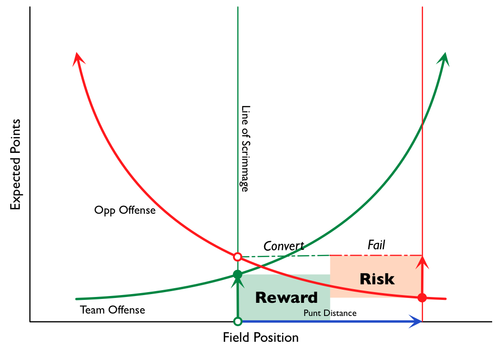
2:28: So here’s something I drew up on my iPad while I was without internet over the weekend.  It’s a generic visualization of a Punt/Go For It decision:

I have a longer post in the works that explains better and uses some actual data, but despite looking complicated, I think it’s actually a pretty simple way of analyzing these situations quickly.  In particular, it lets you adjust for relative team strength and/or type of offense without having to resort to complicated math (you can just “shock” the curves like you would in an econ class).

2:40: “Bills force late INT to finish off fading Eagles” is one of ESPN’s headlines for the Bills/Eagles game.  Not saying Vick didn’t screw the pooch in this one, but as I’ve been harping on the past couple of weeks, if there’s a time to risk throwing an interception, it’s when you’re down by 5 with under 2 minutes left.  If I were the coach and that drive ended with anything other than a touchdown or an interception, I’d be pissed.

2:46: I should make this a TMQ-like running item: “Interception of the Week,” celebrating the game-losing turnovers that happened at the most appropriate time to gamble.  It’s a bit like back when I played a lot of live poker: I used to record my “worst” river calls (where I called with some ridiculously weak hand and ended up being up against a monster), and then I’d brag about them to my friends.

2:51: Man, when did Wes Welker become New England’s “greatest asset”?  I remember when he was on the Dolphins, I thought he was underrated as a situational player, and I was unsurprised to see the Patriots pick him up.  Then his numbers went way up with Randy Moss, which I would have expected, and I kind of thought he got a bit overrated.  But now with Moss in the wind, he’s putting up even bigger numbers.  Crazy.

2:55: So my Quantum Randy Moss post—though the most popular non-Dennis Rodman post I’ve ever written—is one of my least brag-worthy in terms of results: Since I posted it (at the start of last season), Moss had his first 0 catch game, was dumped by two teams, was a non-factor on another, retired in a huff, and reportedly New England wouldn’t even take him back for less money.  I mean, I stand by my analysis, but what an unexpected disaster.

3:15: David Myers: I’ll look into that in a bit.  You could be right that I missed something, but it seemed to work out when I did it on paper.

3:20: So the “Reward” in that graph is the value of your drive times the odds of making the first down, and the “Risk” is the value of the opponent’s drive on the current LoS vs. where they would be expected to get the ball after a punt (times the chances of your failing to convert).  So you’re saying the green arrow on the left should extend to the opp’s drive value curve, but I’m not getting why.

Wouldn’t that be double-counting?

3:30: Nevermind, I get what you’re saying, misread your comment.  You’re saying you should also count denying the opponent a possession at all.  But outside of time-pressure scenarios, I don’t think that has any additional value (aside from what’s already covered in my proportions).

4:07: Argh, I’m getting bogged down in some database mechanics for an idea I was just having.  Note to self: don’t do massive original research projects during the live blog.

4:10: Myers expanded on his comment:

If you punt on play N, then the transition of scoring potential from play N to play N + 1 is from the green solid point to the red solid point, or A + C. The value of the _possession_ in turn has to be the additive inverse of that (plus whatever value is gained by the additional yardage made to get the first). Note this is logically equivalent to the argument about turnover value from The Hidden Game of Football (pp 102-103, 1988 edition). This valuation scheme is not original to me.

I’ll have to postpone looking into this until I have more time (love the academic citation btw).

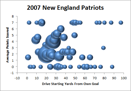
4:52: Ugh, a little less than timely.  I was trying to find a more elegant way of doing this, but here’s a graph of the 2007 Patriots offense:

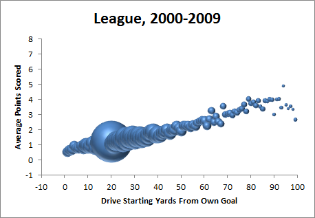
5:07: And here’s the comparison pic:

5:15: FWIW, the linear trendline equations for those two graphs are

and

respectively.

5:20: I just built those graphs from play-by-play data, which I started during the New England game (see, I was trying to reminisce about the crazy 2007 New England offense that you should never ever punt to).  Not only is that game over, but the night game is starting.  Sometimes I definitely overestimate my own speed.

5:23: Short break and I’ll be back with some crazy Aaron Rodgers stats.

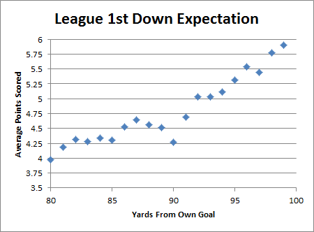
5:40: Ok, quick side-product of what I was doing above: here’s a graph of expected points resulting from a 1st down on each yard line in the red zone:

6:02: Also, I don’t think the variations in that graph are all noise.  First, the sample is pretty huge (n=15,088),  and it’s consistent with other research I’ve done about the bizarre things that happen with a “compressed field.”  Here are some of the features that I can see and the theoretical justifications:

1. There’s a decline right before the 10 yard line, with the 10 yard line itself being a pretty serious local minimum.  I think this happens because of the shortened field and the increasing difficulty of getting a first down without getting a touchdown (e.g., from the 11 yard line, you can only get a first down inside the 1, but from the 13 yard line you have 3 yards to work with).  This is relevant b/c the odds of a touchdown on any given play from the 10, 11, 12 aren’t that different.
2. There’s a flattening that occurs between the 20 and the 15: I think this is where you first experience “compressed field” issues (less room for receivers to run).  But then around the 15, I think the effect is “complete” (at least for a while), and the natural advantage of being closer takes over again.
3. There’s a “statistically significant” outlier on the 3 yard line, where 1st and goal on the 3 is actually less valuable than 1st and goal on the 4.  I’m fairly certain that this at least in part due to configuration issues (as you have limited offensive options on the 3), though I think it may also be caused by poor play selection.  Specifically, teams call a much higher percentage of running plays from the 3 than from the 4, while defenses are pretty much always stacked against the run.
4. The slope at the 10 going down to the 8 is somewhat greater than in other areas of the graph where the expectation is increasing linearly (incidentally, as I mentioned 2 weeks ago, this is one of the things that makes EPA and WPA models difficult: you have some pretty dramatic shifts over a small number of yards, and you can’t really model it with a continuous equation).  This effect I also think might have something to do with play selection, or even 2nd-order play selection: that is, teams pass a fair amount, which is good, running is also fairly effective (b/c defenses are more focused on pass), and successful runs often leave them at a yardline (like the 4+) where they are still willing to pass.

Really, it may seem crazy, but I’ve looked into most of these effects and have found support for them.

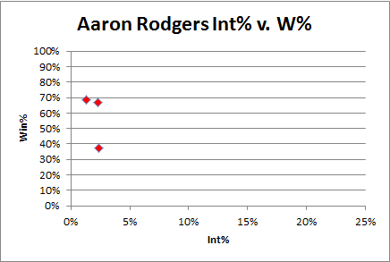
6:36: Ok, as I’ve noted before, Rodgers’ consistently low interception % is pretty unusual, though of course his sample size is tiny:

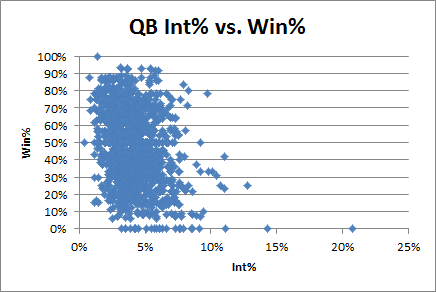
Now let’s compare to the rest of the league (starting at least 8 games):

Obviously he is way on the left side of this blob, and his “slope” (if you can call it that with only 3 points so far) is much higher.

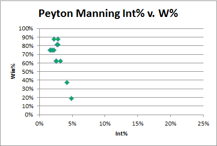
6:40: Let’s compare to Peyton Manning:

Rodgers’ Int% with a 40% win rate is almost half that of Peyton Manning’s (and, it goes without saying, Manning is a pretty consistent QB).

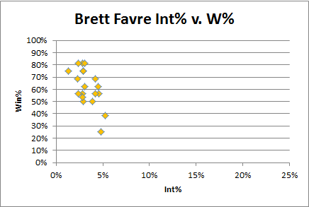
6:45: And, of course, what Rodgers analysis could be complete without comparison to Brett Favre:

6:52: I should note, of course, that I have no problem with Favre or Manning’s numbers here.  I cite Rodger’s consistency not b/c I think it’s necessarily better, but just b/c it’s interesting.  I would expect a QB to have a higher Int% when playing for a losing team, whether he is consistent or not.  Generally, I think a relatively high “shot group” on this graph, with a relatively low slope, can be a good thing: It may simply reflect that the QB is taking necessary risks when required to (though, clearly, isolating the causes and effects is incredibly difficult).

7:00: I see Tiger Woods bounced back with three 68’s in a row in the Frys.com tournament.  He finished tied for 30th.  In what is basically a “Quest for the Card” tournament.  In a field that contained 9 of the world’s top 100 players.

Comeback?

7:15: Atlanta is such a sneaky franchise. They seem to be competitive every couple of years, putting together good-to-great regular seasons, but haven’t won more than one playoff game since 1998.  I think you can win with great passing and great running, great defense and great running, but you can’t win with great running alone.  Their performance, to me, seems like a classic run good/run bad situation, where they probably haven’t changed all that much year to year, but being a little better than average keeps them occasionally in contention (while still being at a disadvantage against the actually better teams that they have to face in the playoffs).

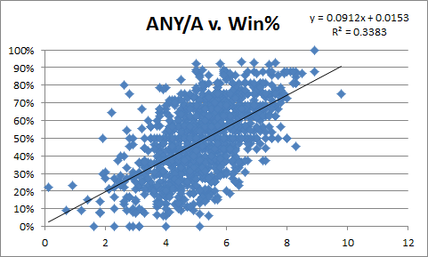
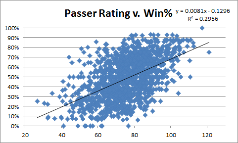
7:42: Rodgers has a sick Adjusted Net Yards Per Attempt (generally considered the best non–play-by-play single QB metric) this season, leading the league with 9.7 going into this weekend.

So, out of curiosity, I was kind of curious just how much better ANY/A is than the pariah of QB stats: the NFL Passer Rating.  So here are a couple of simple scatter-plots, ANY/A first:

And here’s PER:

ANY/A obv does better, though maybe not as much as I would have guessed.

7:47: Of course, both stats are subject to causation/entanglement issues, ANY/A possibly even moreso (as it includes sacks and weights interceptions more heavily).

7:54: That style of touchdown where a receiver has one defender, breaks for the sideline, then turns, leaps and stretches out for the touchdown, is always hailed as a great play, despite being completely textbook and despite being executed pretty much exactly the same way by every receiver in the NFL—normally differing only by whether they are close enough and have a good enough angle to get inside the pylon.

7:58: Man, I’m excited for Detroit/Chicago tomorrow.  Can’t remember the last time I thought that.

8:14: Ok, I can’t help but return to this David Myers point from earlier:

If you punt on play N, then the transition of scoring potential from play N to play N + 1 is from the green solid point to the red solid point, or A + C. The value of the _possession_ in turn has to be the additive inverse of that (plus whatever value is gained by the additional yardage made to get the first).

I don’t think the possession has value in addition to its scoring potential, or at least not as much as you’re suggesting.  This method you’re describing counts the value of not giving the opponent the ball in addition to the value of keeping the ball for yourself.  But I really think you shouldn’t do that, since you haven’t decreased the expected possessions for the game of your opponent—or, at least, you certainly haven’t decreased it by 1.  They are still going to get the ball when your possession is over.  By holding the ball now, you make it slightly more likely that the last drive of the game will be yours (depending on how much time is left, etc), but you’re still going to be trading possessions 1 for 1.

For an analogy, think of rebounding in basketball: Occasionally I’ve heard casual fans suggest that offensive rebounds must be more important than defensive rebounds because you not only get a possession but you take one away from your opponent.  But this is strictly false: A rebound is worth one possession regardless (note, of course, offensive rebounds probably are more valuable than defensive rebounds, but only because you are less likely to get them).  What you gain by getting an offensive rebound is exactly your expectation for your new possession, b/c the other team is still going to get the ball back when it’s over.  I can’t see any distinction between this and converting a 4th down.

8:24: Also, it’s true that, depending on where you are on the field, your opponent may be expected to get the ball back in a worse position.  But this effect should be included in whatever you use for value on the Y-axis.  At least, a perfect metric for the Y-axis would include it (though I think a proxy like expected points is good enough for most approximations, which is what that graphing method is all about).

8:29: Wow, can’t wait for that Packers/Chargers game.

8:32: Game, set, match.  Respect to Aaron Rodgers for breaking a Kurt Warner record (PER over first 1500 attempts).  Was there anything more incredible in the history of football than the 1999 Rams?