In the conventional wisdom, winning is probably overrated. The problem ultimately boils down to information quality: You only get one win or loss per game, so in the short-run, great teams, mediocre team, or teams that just get lucky can all achieve the same results. Margin of victory, on the other hand, has a whole range of possible outcomes that, while imperfectly descriptive of the bottom line, correlate strongly with team strength. You can think about it like sample size: a team’s margin of victory over a handful of games gives you a lot more data to work with than their won-loss record. Thus, particularly when the number of games you draw your data from is small, MOV tends to be more probative.
Long ago, the analytic community recognized this fact, and has moved en masse to MOV (and its ilk) as the main element in their predictive statistics. John Hollinger, for example, uses margin exclusively in his team power ratings—completely ignoring winning percentage—and these ratings are subsequently used for his playoff prediction odds, etc. Note, Hollinger’s model has a lot of baffling components, like heavily weighting a team’s performance in their last 10 games (or later in their last 25% of games), when there is no statistical evidence that L10 is any more predictive than first 10 (or any other 10). But this particular choice is of particular interest, especially as it is indicative of an almost uniform tendency among analysts to substitute MOV-style stats for winning percentage entirely.
This is both logically and empirically a mistake. As your sample size grows, winning percentage becomes more and more valuable. The reason for this is simple: Winning percentage is perfectly accurate—that is, it perfectly reflects what it is that we want to know—but has extremely high variance, while MOV is an imperfect proxy, whose usefulness stems primarily from its much lower variance. As sample sizes increase, the variance for MOV decreases towards 0 (which happens relatively quickly), but the gap between what it measures and what we want to know will persist in perpetuity. Thus, after a certain point, the “error” in MOV remains effectively constant, while the “error” in winning percentage continuously decreases. To get a simple intuitive sense of this, imagine the extremes: after 5 games, clearly you will have more faith in a team that has won 2 but has a MOV of +10 over a team that has won 3 but has a MOV of +1. But now imagine 1000 games with the same MOV’s and winning percentages: one team has won 400 and the other has won 600. If you had to place money on one of the two teams to win their next game, you would be a fool to favor the first. But beyond the intuitive point, this is essentially an empirical matter: with sufficient data, we should be able to establish the relative importance of each for any given sample-size.
So for this post, I’ve employed the same method that I used in section (b) to create our MOV-> Win% formula (logistic regression for all 55,000+ team games since 1986), except this time I included both Win % and MOV (over the team’s other 81 games) as the predictive variables. Here, first, are the coefficients and corresponding p-values (probability that the variable is not significant):

It is thus empirically incontrovertible that, even with an 81-game predictive sample, both MOV and Win% are statistically significant predictive factors. Also, for those who don’t eat logistic regression outputs for breakfast, I should be perfectly clear what this means: It doesn’t just mean that both W% and MOV are good at predicting W%—this is trivially true—it means that, even when you have one, using the other as well will make your predictions substantially better. To be specific, here is the formula that you would use to predict a team’s winning percentage based on these two variables:
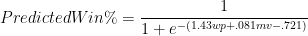
Note: Again, e is euler’s number, or ~2.72. wp is the variable for winning % over the other 81 games, and mv is the variable for Margin of Victory over the other 81 games.
And again, for your home-viewing enjoyment, here is the corresponding Excel formula:
=1/(1+EXP(-(1.43*[W%]+.081[MOV]-.721)))
Finally, in order to visualize the relative importance of each variable, we can look at their standardized coefficients (shown here with 95% confidence bars):

Note: Standardized coefficients, again, are basically a unit of measurement for comparing the importance of things that come in different shapes and sizes.
For an 81-game sample (which is about as large of a consistent sample as you can get in the NBA), Win% is about 60% as important as MOV when it comes to predicting outcomes. At the risk of sounding redundant, I need to make this extremely clear again: this does NOT mean that Win% is 60% as good at predicting outcomes as margin of victory (actually, it’s more like 98% as good at that)—it means that, when making your ideal prediction, which incorporates both variables, Win % gets 60% as much weight as MOV (as an aside, I should also note that the importance of MOV drops virtually to zero when it comes to predicting playoff outcomes, largely—though not entirely—because of home court advantage).
This may not sound like much, but I think it’s a pretty significant result: At the end of the day, this proves that there IS a skill to winning games independent of the rates at which you score and allow points. This is a non-obvious outcome that is almost entirely dismissed by the analytical community. If NBA games were a random walk based on possession-to-possession reciprocal advantages, this would not be the case at all.
Now, note that this is formally the same as the scenario discussed in section (b): We want to predict winning percentages, but using MOV alone leaves a certain amount of error. What this regression proves is that this error can be reduced by incorporating win percentage into our predictions as well. So consider this proof-positive that X-factors are predictively valuable. Since the predictive power of Win% and MOV should be equivalent no matter their source, we can now use this regression to make more accurate predictions about each player’s true impact.
Adapting this equation for individual player use is simple enough, though slightly different from before: Before entering the player’s Win% differential, we have to convert it into a raw win percentage, by adding .5. So, for example, if a player’s W% differential were 21.6%, we would enter 71.6%. Then, when a number comes out the other side, we can convert it back into a predicted differential by subtracting .5, etc.
Using this method, Rodman’s predicted win differential comes out to 14.8%. Here is the new histogram:

Note: N is still 470.
This histogram is also weighted by the sample size for each player (meaning that a player with 100 games worth of qualifying minutes counts as 100 identical examples in a much larger dataset, etc.). I did this to get the most accurate distribution numbers to compute P values (which, in this case, work much like a percentile) for individual players. Here is a summary of the major factors for Dennis Rodman:

For comparison, I’ve also listed the percentage of eligible players that match the qualifying thresholds of my dataset (minus the games missed) who are in the Hall of Fame. Specifically, that is, those players who retired in 2004 or earlier and who have at least 3 seasons since 1986 with at least 15 games played in which they averaged at least 15 minutes per game. This gives us a list of 462 players, of which 23 are presently IN the Hall. The difference in average skill between that set of players and the differential set is minimal, and the reddish box on the histogram above surrounds the top 5% of predicted Win% differentials in our main data.
While we’re at it, let’s check in on the list of “select” players we first saw in section (a) and how they rank in this metric, as well as in some of the others I’ve discussed:

For fun, I’ve put average rank and rank of ranks (for raw W% diff, adjusted W% diff, MOV-based regression, raw W%/MOV-based regression, raw X-Factor, adjusted X-Factor, and adjusted W%/MOV-based regression) on the far right. I’ve also uploaded the complete win differential table for all 470 players to the site, including all of the actual values for these metrics and more. No matter which flavor of metric you prefer (and I believe the highlighted one to be the best), Rodman is solidly in Hall of Fame territory.
Finally, I’m not saying that the Hall of Fame does or must pick players based on their ability to contribute to their team’s winning percentages. But if they did, and if these numbers were accurate, Rodman would deserve a position with room to spare. Thus, naturally, one burning question remains: how much can we trust these numbers (and Dennis Rodman’s in particular)? This is what I will address in section (d) tomorrow.
If combining win % and MOV is a better indicator of the next win, would it also make a more accurate “ranking” then Hollinger’s system?
Actually, Win% alone is more accurate than Hollinger’s system. So yeah, this would be even better.
Cool, if that interview went well, and you end up being the “hollinger” at another site, I hope you do your daily rankings that way.
I assume that MOV as an independent variable attenuates, due to the strategic or other differences that occur when a team is ahead or behind by a large margin in the 4th quarter.
Is there a way to control for this, perhaps by defining “blowout” (say, MOV of 20+) and then pulling the count of blowouts out as a third independent variable?
m
Wow, this is awesome stuff.
One objection: concerning your regression of WIN% on MOV and WIN%, are you sure you aren’t facing a multicollinearity problem?
As I’m sure you’re aware, this will not affect the predictive power of the model, but will make interpretations of the coefficients of the independent variables suspect. So, concluding that WIN% gets sixty percent of the weight that MOV does in prediction is probably inaccurate.
For what it’s worth, the correlation between MOV and WIN% for the 2010-2011 season is 0.971–strong enough to present interpretation issues for your model.
I’ve been working on how to account for MOV and Win% “separately” for a long time and will have a new series on the subject coming out shortly.
Props, though, for pointing out a legitimate weakness. I do think my analysis in this section of the Rodman series is somewhat lacking (as is my extremely rudimentary treatment of “adjusted” win percentage), especially compared to the research I’ve been working on more recently. If I ever re-publish this thing, it will need some refining.
Fortunately though, most of these issues are matters of detail, and don’t impact the underlying conclusions.
Great. Looking forward to your new posts!