The many histograms in sections (a)-(c) of Part 3 reflect fantastic p-values (probability that the outcome occurred by chance) for Dennis Rodman’s win percentage differentials relative to other players, but, technically, this doesn’t say anything about the p-values of each metric in itself. What this means is, while we have confidently established that Rodman’s didn’t just get lucky in putting up better numbers than his peers, we haven’t yet established the extent to which his being one of the best players by this measure actually proves his value. This is probably a minor distinction to all but my most nitpicky readers, but it is exactly one of those nagging “little insignificant details” that ends up being a key to the entire mystery.
The Technical Part (Feel Free to Skip)
The challenge here is this: My preferred method for rating the usefulness and reliability of various statistics is to see how accurate they are at predicting win differentials. But, now, the statistic I would like to test actually is win differential. The problem, of course, is that a player’s win differential is always going to be exactly identical to his win differential. If you’re familiar with the halting problem or Gödel’s incompleteness theorem, you probably know that this probably isn’t directly solvable: that is, I probably can’t design a metric for evaluating metrics that is capable of evaluating itself.
To work around this, our first step must be to independently assess the reliability of win predictions that are based on our inputs. As in sections (b) and (c), we should be able to do this on a team-by-team basis and adapt the results for player-by-player use. Specifically, what we need to know is the error distribution for the outcome-predicting equation—but this raises its own problems.
Normally, to get an error distribution of a predictive model, you just run the model a bunch of times and then measure the predicted results versus the actual results (calculating your average error, standard deviation, correlation, whatever). But, because my regression was to individual games, the error distribution gets “black-boxed” into the single-game win probability.
[A brief tangent: “Black box” is a term I use to refer to situations where the variance of your input elements gets sucked into the win percentage of a single outcome. E.g., in the NFL, when a coach must decide whether to punt or go for it on 4th down late in a game, his decision one way or the other may be described as “cautious” or “risky” or “gambling” or “conservative.” But these descriptions are utterly vapid: with respect to winning, there is no such thing as a play that is more or less “risky” than any other—there are only plays that improve your chances of winning and plays that hurt them. One play may seem like a bigger “gamble,” because there is a larger immediate disparity between its possible outcomes, but a 60% chance of winning is a 60% chance of winning. Whether your chances comes from superficially “risky” plays or superficially “cautious” ones, outside the “black box” of the game, they are equally volatile.]
For our purposes, what this means is that we need to choose something else to predict: specifically, something that will have an accurate and measurable error distribution. Thus, instead of using data from 81 games to predict the probability of winning one game, I decided to use data from 41 season-games to predict a team’s winning percentage in its other 41 games.
To do this, I split every team season since 1986 in half randomly, 10 times each, leading to a dataset of 6000ish randomly-generated half-season pairs. I then ran a logistic regression from each half to the other, using team winning percentage and team margin of victory as the input variables and games won as the output variable. I then measured the distribution of those outcomes, which gives us a baseline standard deviation for our predicted wins metric for a 41 game sample.
Next, as I discussed briefly in section (b), we can adapt the distribution to other sample sizes, so long as everything is distributed normally (which, at every point in the way so far, it has been). This is a feature of the normal distribution: it is easy to predict the error distribution of larger and smaller datasets—your standard deviation will be directly proportional to the square-root of the ratio of the new sample size to the original sample size.
Since I measured the original standard deviations in games, I converted each player’s “Qualifying Minutes” into “Qualifying Games” by dividing by 36. So the sample-size-adjusted standard deviation is calculated like this:
Since the metrics we’re testing are all in percentages, we then divide the new standard deviation by the size of the sample, like so:
This gives us a standard deviation for actual vs. predicted winning percentages for any sample size. Whew!
The Good, Better, and Best Part
The good news is: now that we can generate standard deviations for each player’s win differentials, this allows us to calculate p-values for each metric, which allows us to finally address the big questions head on: How likely is it that this player’s performance was due to chance? Or, put another way: How much evidence is there that this player had a significant impact on winning?
The better news is: since our standard deviations are adjusted for sample size, we can greatly increase the size of the comparison pool, because players with smaller samples are “punished” accordingly. Thus, I dropped the 3-season requirement and the total minutes requirement entirely. The only remaining filters are that the player missed at least 15 games for each season in which a differential is computed, and that the player averaged at least 15 minutes per game played in those seasons. The new dataset now includes 1539 players.
Normally I don’t weight individual qualifying seasons when computing career differentials for qualifying players, because the weights are an evidentiary matter rather than an impact matter: when it comes to estimating a player’s impact, conceptually I think a player’s effect on team performance should be averaged across circumstances equally. But this comparison isn’t about whose stats indicate the most skill, but whose stats make for the best evidence of positive contribution. Thus, I’ve weighted each season (by the smaller of games missed or played) before making the relevant calculations.
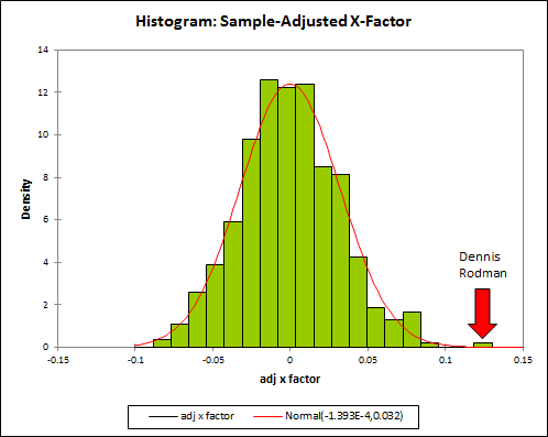
So without further ado, here are Dennis Rodman’s statistical significance scores for the 4 versions of Win % differential, as well as where he ranks against the other players in our comparison pool:

Note: I’ve posted a complete table of z scores and p values for all 1539 players on the site. Note also that due to the weighting, some of the individual differential stats will be slightly different from their previous values.
You should be careful to understand the difference between this table of p-values and ranks vs. similar ones from earlier sections. In those tables, the p-value was determined by Rodman’s relative position in the pool, so the p-value and rank basically represented the same thing. In this case, the p-value is based on the expected error in the results. Specifically, they are the answer to the question “If Dennis Rodman actually had zero impact, how likely would it be for him to have posted these differentials over a sample of this size?” The “rank” is then where his answer ranks among the answers to the same question for the other 1538 players. Depending on your favorite flavor of win differential, Rodman ranks anywhere from 1st to 8th. His average rank among those is 3.5, which is 2nd only to Shaquille O’Neal (whose differentials are smaller but whose sample is much larger).
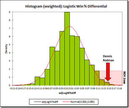
Of course, my preference is for the combined/adjusted stat. So here is my final histogram:

Note: N=1539.
Now, to be completely clear, as I addressed in Part 3(a) and 2(b), so that I don’t get flamed (or stabbed, poisoned, shot, beaten, shot again, mutilated, drowned, and burned—metaphorically): Yes, actually I AM saying that, when it comes to empirical evidence based on win differentials, Rodman IS superior to Michael Jordan. This doesn’t mean he was the better player: for that, we can speculate, watch the tape, or analyze other sources of statistical evidence all day long. But for this source of information, in the final reckoning, win differentials provide more evidence of Dennis Rodman’s value than they do of Michael Jordan’s.
The best news is: That’s it. This is game, set, and match. If the 5 championships, the ridiculous rebounding stats, the deconstructed margin of victory, etc., aren’t enough to convince you, this should be: Looking at Win% and MOV differentials over the past 25 years, when we examine which players have the strongest, most reliable evidence that they were substantial contributors to their teams’ ability to win more basketball games, Dennis Rodman is among the tiny handful of players at the very very top.
So according to this method, Eddie Jones is the 4th best player since 1986?
4th best evidence of goodness.
That’s essentially the same thing right? What do you think about your results contradicting common beliefs? That the truth is somewhere in between? We need more research? What do the top people on your list have in common?
1. No.
2. Where the “contradiction” is a severe and genuine disagreement—e.g., if there is someone people thought was good (Mookie Blaylock) but my model says there is strong evidence that they were bad, or vice versa—I would trust my model.
3. There should be a strong but not perfect correlation between actual goodness and evidence of goodness.
4. Always.
5. This (or something similar) is prob my next area of research. I’m building a model for player value that is rooted in the correlation between evidence of winning impact and various statistical profiles.
I guess I’m not grasping this right. If one player has the most evidence of goodness, doesn’t that mean he is the best player according to this method?
No. Think of it like so: This method combines how good the data says a player is (based on win differentials alone) with how reliable his data is (based on amount of qualifying time), with the end result being how much differentials tells us about the probability that he was a good player.
So, someone could be a moderately good player but have a huge amount of qualifying data, and they can do as well as someone who is an incredible player but has a much smaller amount of qualifying time. Note, for example, that Larry Bird ranks 5th despite having only two qualifying seasons in his sample.
Ooohh. Wow. I was forgetting that not every season was included. I was thinking of it like the +/- we have now.
For win differentials yes, Rodman had more value in the seasons he qualified in, but that is all you could say from this. For instance, MJ has only 2 seasons of data and one was his second year and one was when he was with the Wizards. Is there a way to overcome this bias? I understand that using Win Differentials and MOV you can only use the seasons when a player missed more than 15 games but it seems a little biased to compare player to player. I think Rodman’s overall value is without question but I just have doubts about comparing player to player.
I think player to player comparisons are fine as long as it is properly understood what is being measured and how much uncertainty their is: in no way should this method be considered the ultimate arbitrator for all player value disputes. However, it can still provide a lot of insight, both as supplementary info about particular players, and for identifying league-trends and such.
I respect your articles. I think you’ve done n INCREDIBLE job. You’ve definitely shown Rodman has elite value. Which satisfies the DR fan in me. I must ask though: Don’t you think (considering the two seasons that we’re used to represent Jordan) that it is misleading to say that “Rodman IS superior to Michael Jordan.”?
Maybe I should be slightly less coy about this: I do NOT believe that Rodman was a better player than Michael Jordan. Indeed, no one is. All I mean is that, when it comes to win differentials, there is a greater amount of evidence in Rodman’s favor. This is true precisely because Jordan has so little qualifying data overall (or at least mostly so). If players have less data, it doesn’t necessarily mean they aren’t as good, it just means you have to look to other sources.
Forgive my ignorance, but why does Jordan have only two qualifying seasons since 1986?
Qualifying seasons require having missed and played at least 15 regular-season games for the same team in the same year. Jordan did this in his comeback year of 94-95, and again in his first season with the wizards in 2001-2002. He also played a limited number of minutes in small number of games in 1985-86, but it’s probably for the better that my sample doesn’t go back that far, as I doubt they would be representative.
I’m a big Rodman fan and this whole series goes with my long held beliefs about basketball and Rodman, BUT this particular analysis just tells us that Rodman and Shaq were some of the best players to miss a lot of games during their best seasons.
Great players that missed few games during their good seasons are not included.
Yes, like I said early on, it’s a pity we don’t force all players to sit out every other night and uniformly rotate teams over the course of their careers, so that me might more accurately evaluate their value.
Some one else things Dennis Rodman is an elite player! http://arturogalletti.wordpress.com/2011/03/16/nerd-numbers-guest-post-top-25-players-part-two/
What do you think of the Wins Produced player evaluation?
Have you read about adjusted rebounding? Any comments?
Some links here http://stats-for-the-nba.appspot.com/
Some discussion here http://sonicscentral.com/apbrmetrics/viewforum.php?f=1
Separate from that, I agree with
1) non-linear stat impacts and the desirability of dynamic models
2) models that capture player win impacts at game level over season level and game win impacts over raw game impacts or aggregate season impacts.
I am not familiar with “adjusted rebounding” (at least, not by that name), but I’ll look into it.
I wonder, is it possible that Rodman’s value is somewhat overrated by this method due to the type of reasons for missing games? I would expect the two main reasons for qualifying are trades and injuries, and both should downplay the value of the player. However, in Rodman’s case I would guess that suspensions have a major part as well. Do you think it’s reasonable that this will have an effect? I don’t think it would be a major effect, but it seems like something to consider.
I was concerned about this kind of thing generally, so I tried looking into the difference in a player’s win-rates before and after the time that they missed, and didn’t find a significant drop. Interestingly, though, I’ve found that a player’s box-score-based “contributions” tend to drop significantly after missing time, even when their winrates appear to remain fairly steady. This generally backs up my theory that box-score stats describe a player’s role much more than they measure his impact.
For trades, I’ve looked at a smallish sample, and the win differentials do tend to be a little less reliable than when they come from injuries or suspension, with the effect strongest for mediocre players. I think this is because most trades with high quality players are pretty lopsided by design. If anything, late-season trades of quality players may actually skew their results in the other direction, as the team they are leaving is frequently blowing itself up to rebuild while the other is filling essential holes for a playoff run, etc.