ESPN Stat Geek Smackdown 2011 Champion

. . . is me.

Final Standings:

Benjamin Morris (68)
Stephen Ilardi (65)
Matthew Stahlhut (56)
(Tie) Haralabos Voulgaris (54)
(Tie) John Hollinger (54)
David Berri (52)
Neil Paine (49)
Henry Abbott’s Mom (46)

To go totally obscure, I feel like Packattack must have felt when he pulled off this strat (the greatest in the history of Super Monkey Ball):

That is, he couldn’t have done it without a lot of luck, but it still feels better than just getting lucky.

As for the result, I don’t have any awesome gloating comments prepared: Like all the other “Stat Geeks,” I thought Miami was a favorite going into the Finals—and given what we knew then, I would think that again. But at this point I definitely feel like the better team won.

For as far as they went, Miami’s experiment of putting 3 league-class primary options on the same team was essentially a failure. I’m sure the narrative will be about how they were “in disarray” or needed more time together, but ultimately it’s a design flaw. Without major changes, I think they’ll be in a similar spot every year: that is, they’ll be very good, and maybe even contenders, but they won’t ever be the dominant team so many imagined.

As for Dallas, they played beautiful basketball throughout the playoffs, and I personally love seeing a long-range shooting team take it down for a change. It’s noteworthy that they defied two of the patterns I identified in my “How to Win a Championship in Any Sport” article: They become only the second NBA team since 2000 with a top-3 payroll to win it all, and they’re only the second champion in 21 years without a first-team All-NBA player.

Bayes’ Theorem, Small Samples, and WTF is Up With NBA Finals Markets?

Seriously, I am dying to post about something non-NBA related, and I should have my Open-era tennis ELO ratings by surface out in the next day or so. But last night I finally got around to checking the betting markets to see how the NBA Finals—and thus my chances of winning the Smackdown—were shaping up, and I was shocked by what I found. Anyway, I tossed a few numbers around, and thought you all might find them interesting. Plus, there’s a nice little object-lesson about the usefulness of small sample size information for making Bayesian inferences. This is actually one area where I think the normal stat geek vs. public dichotomy gets turned on its head: Most statistically-oriented people reflexively dismiss any empirical evidence without a giant data-set. But in certain cases—particularly those with a wide range of coherent possibilities—I think the general public may even be a little too conservative about the implications of seemingly minor statistical anomalies.

Freaky Finals Odds:

First, I found that most books seem to see the series as a tossup at this point. Here’s an example from a European sports-betting market:

Intuitively, this seemed off to me. Dallas needs to win 1 out of the 2 remaining games in Miami. Assuming the odds for both games are identical (admittedly, this could be a dubious assumption), here’s a plot of Dallas’s chances of winning the series relative to Miami’s expected winrate per home game:

So for the series to be a tossup, Miami needs to be about a 71% favorite per game. Even at home in the playoffs, this is extremely high. Depending on what dataset you use, the home team wins around 60-65% of the time in the NBA regular season and about 65%-70% of the time in the postseason. But that latter number is a bit deceptive, since the playoffs are structured so that more games are played in the homes of the better teams: aside from the 2-3-2 Finals, any series that ends in an odd number of games gives the higher-seeded team (who is often much better) an extra game at home. In fact, while I haven’t looked into the issue, that extra 5% could theoretically be less than the typical skill-disparity between home and away teams in the playoffs, which would actually make home court less advantageous than in the regular season.

Now, Miami has won only 73% of their home games this season, and it was against below-average competition (overall, they had one of the weakest schedules in the league). Counting the playoffs, at this point Dallas actually has a better record than Miami (by one game), and they played an above-average schedule. More importantly, the Mavs won 68% of their games on the road (compare to the league average of 35-40%). Not to mention, Dallas is 5-2 against the Heat overall, and 2-1 against them at home (more on that later).

So how does the market tilt so heavily to this side? Honestly, I have no idea. Many people are much more willing to dismiss seemingly incongruent market outcomes than I am. While I obviously think the market can be beaten, when my analytical results diverge wildly from what the money says, my first inclination is to wonder what I’m doing wrong, as the odds of a massive market failure are probably lower than the odds that I made a mistake. But, in this case, with comparatively few variables, I don’t really get it.

It is a well-known phenomenon in sports-betting that huge games often have the juiciest (i.e., least efficient) lines. This is because the smart money that normally keeps the market somewhat efficient can literally start to run out. But why on earth would there be a massive, irrational rush to bet on the Heat? I thought everyone hated them!

Fun With Meta-Analysis:

So, for amusement’s sake, let’s imagine a few different lines of reasoning (I’ll call them “scenarios”) that might lead us to a range of different conclusions about the present state of the series:

Miami won at Home ~73% of the time while Dallas won on the road (a fairly stunning) 68% of the time. If these values are taken at face value, a generic Miami Home team would be roughly 5% better than a generic Dallas road team, making Miami a 52.5% favorite in each game.
The average home team in the NBA wins about 63% of the time. Miami and Dallas seem pretty evenly matched, so Miami should win each game ~63% of the time as well.
Let’s go with the very generous end of broader statistical models (discounting early-season performance, giving Miami credit for championship experience, best player, and other factors), and assume that Miami is about 5-10% better than Dallas on a neutral site. The exact math on this is complicated (since winning is a logistic function), but, ballpark, this would translate into about a 65.5% chance at home.
Markets rule! Approximate Market Price for a Miami series win is ~50%, translating into the 71% chance mentioned above above.

Here’s a scatter-plot of the chances of Dallas winning the series based on those per-game estimates:

Ignore the red dots for now—we’ll get back to those. The blue dots are the probability of Dallas winning at least one of the next two games (using the same binomial formula as the function above). Now, hypothetically, let’s assume you thought each of these analyses were equally plausible, your overall probability for Dallas winning the title would simply be the average of the four scenario’s results, or right around 60%. Note: I am NOT endorsing any of these lines of reasoning or any actual conclusions about this series here—it’s just a thought experiment.

A Little Bayesian Inference:

As I mentioned above, the Mavericks are 5-2 against the Heat this season, including 2-1 against them in Miami. Let’s focus on the second stat: Sticking with the assumption that you found each of these 4 lines of reasoning equally plausible prior to knowing Dallas’s record in Miami, how should your newly-acquired knowledge that they were 2-1 affect your assessment?

Well, wow! 3 games is such a miniscule sample, it can’t possibly be relevant, right? I think most people—stat geek and layperson alike—would find this statistical event pretty unremarkable. In the abstract, they’re right: certainly you wouldn’t let such a thing invalidate a method or process built on an entire season’s worth of data. Yet, sometimes these little details can be more important than they seem. Which brings us to perhaps the most ubiquitously useful tool discovered by man since the wheel: Bayes’ Theorem.

Bayes’ Theorem, at it’s heart, is a fairly simple conceptual tool that allows you to do probability backwards: Garden-variety probability involves taking a number of probabilistic variables and using them to calculate the likelihood of a particular result. But sometimes you have the result, and would like to know how it affects the probabilities of your conditions: Bayesian analysis makes this possible.

So, in this case, instead of looking at the games or series directly, we’re going to look at the odds of Dallas pulling off their 2-1 record in Miami under each of our scenarios above, and then use that information to adjust the probabilities of each. I’ll go into the detail in a moment, but the relevant Bayesian concept is that, given a result, the new probability of each precondition will be adjusted proportionally to its prior probability of producing that result. Looking at the red dots above (which are technically the cumulative binomial probability of Miami winning 0 or 1 out of 3 games), you should see that Dallas is far more likely to go 2-1 or better on Miami’s turf if they are an even match than if Miami is a huge favorite—over twice as likely, in fact. Thus, we should expect that scenarios suggesting the former will become much more likely, and scenarios suggesting the latter will become much less so.

In its simplest form, Bayes’ Theorem states that the probability of A given B is equal to the probability of B given A times the prior probability of A (probability before our new information), divided by the prior probability of B:

$P(A|B)= \frac{P(B|A)*P(A)} {P(B)}$

Though our case looks a little different from this, it is actually a very simple example. First, I’ll treat the belief that the four analyses are equally likely to be correct as a “discrete uniform distribution” of a single variable. That sounds complicated, but it simply means that there are 4 separate options, one of which is actually correct, and each of which is equally likely. Thus, the odds of any given scenario are expressed exactly as above (B is the 2-1 outcome):

$P(S_x)= \frac{P(B|S_x)*P(S_x)} {P(B)}$

The prior probability for S_xis .25. The prior probability of our result (the denominator) is simply the sum of the probabilities of each scenario producing that result, weighted by each scenario’s original probability. But since these are our only options and they are all equal, that element will factor out, as follows:

$P(B)= P(S_x)*(P(B|S_1)+P(B|S_2)+P(B|S_3)+P(B|S_4))$

Since P(S_x) appears in both the numerator and the denominator, it cancels out, leaving our probability for each scenario as follows:

$P(S_x)= \frac{P(B|S_x)} {P(B|S_1)+P(B|S_2)+P(B|S_3)+P(B|S_4)}$

The calculations of P(B|S_x) are the binomial probability of Dallas winning exactly 2 out of 3 games in each case (note this is slightly different from above, so that Dallas is sufficiently punished for not winning all 3), and Excel’s binom.dist() function makes this easy. Plugging those calculations in with everything else, we get the following adjusted probabilities for each scenario:

Note that the most dramatic changes are in our most extreme scenarios, which should make sense both mathematically and intuitively: going 2-1 is much more meaningful if you’re a big dog.

Our new weighted average is about 62%, meaning the 2-1 record improves our estimate of Dallas’s chances by 2%, making the gap between the two 4%: 62-38 (24% difference) instead of 60-40. That may not sound like much, but a few percentage points of edge aren’t that easy to come by. For example, to a gambler, that 4% could be pretty huge: you normally need a 5% edge to beat the house (i.e., you have to win 52.5% of the time), so imagine you were the only person in the world who knew of Dallas’s miniature triumph—in this case, that info alone could get you 80% of the way to profit-land.

Making Use:

I should note that, yes, this analysis makes some massively oversimplifying assumption—in reality, there can be gradients of truths between the various scenarios, with a variety of interactions and hidden variables, etc.—but you’d probably be surprised by how similar the results are whether you do it the more complicated way or not. One of the things that makes Bayesian inference so powerful is that it often reveals trends and effects that are relatively insulated from incidental design decisions. I.e., the results of extremely simplified models are fairly good approximations of those produced by arbitrarily more robust calculations. Consequently, once you get used to it, you will find that you can make quick, accurate, and incredibly useful inferences and estimates in a broad range of practical contexts. The only downside is that, once you get started on this path, it’s a bit like getting Tetrisized: you start seeing Bayesian implications everywhere you look, and you can’t turn it off.

Of course, you also have to be careful: despite the flexibility Bayesian analysis provides, using it in abstract situations—like a meta-analysis of nebulous hypotheses based on very little new information—is very tricky business, requiring good logical instincts, a fair capacity for introspection, and much practice. And I can’t stress enough that this is a very different beast from the typical talking head that uses small samples to invalidate massive amounts of data in support of some bold, eye-catching and usually preposterous pronouncement.

Finally, while I’m not explicitly endorsing any of the actual results of the hypo I presented above, I definitely think there are real-life equivalents where even stronger conclusions can be drawn from similarly thin data. E.g., one situation that I’ve tested both analytically and empirically is when one team pulls off a freakishly unlikely upset in the playoffs: it can significantly improve the chances that they are better than even our most accurate models (all of which have significant error margins) would indicate.

Game Theory in Practice: Smackdown Meta-Strategy

Going into the final round of ESPN’s Stat Geek Smackdown, I found myself 4 points behind leader Stephen Ilardi, with only 7 points left on the table: 5 for picking the final series correctly, and a bonus 2 for also picking the correct number of games. The bottom line being, the only way I could win is if the two of us picked opposite sides. Thus, with Miami being a clear (though not insurmountable) favorite in the Finals, I picked Dallas. As noted in the ESPN write-up”

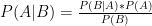
“The Heat,” says Morris, “have a better record, home-court advantage, a better MOV [margin of victory], better SRS [simple rating system], more star power, more championship experience, and had a tougher road to the Finals. Plus Miami’s poor early-season performance can be fairly discounted, and it has important players back from injury. Thus, my model heavily favors Miami in five or six games.

But I’m sure Ilardi knows all this, so, since I’m playing to win, I’ll take Dallas. Of course, I’m gambling that Ilardi will play it safe and stick with Miami himself since I’m the only person close enough to catch him. If he assumes I will switch, he could also switch to Dallas and sew this thing up right now. Game-theoretically, there’s a mixed-strategy Nash equilibrium solution to the situation, but without knowing any more about the guy, I have to assume he’ll play it like most people would. If he’s tricky enough to level me, congrats.

Since I actually bothered to work out the equilibrium solution, I thought some of you might be interested in seeing it. Also, the situation is well-suited to illustrate a couple of practical points about how and when you should incorporate game-theoretic strategies in real life (or at least in real games).

Some Game Theory Basics

Certainly many of my readers are intimately familiar with game theory already (some probably much more than I am), but for those who are less so, I thought I should explain what a “mixed-strategy Nash equilibrium solution” is, before getting into the details on the Smackdown version (really, it’s not as complicated as it sounds).

A set of strategies and outcomes for a game is an “equilibrium” (often called a “Nash equilibrium”) if no player has any reason to deviate from it. One of the most basic and most famous examples is the “prisoner’s dilemma” (I won’t get into the details, but if you’re not familiar with it already, you can read more at the link): the incentive structure of that game sets up an equilibrium where both prisoners rat on each other, even though it would be better for them overall if they both kept quiet. “Rat/Rat” is an equilibrium because an individual deviating from it will only hurt themselves. Bother prisoners staying silent is NOT an equilibrium, because either can improve their situation by switching strategies (note that games can also have multiple equilibriums, such as the “Which Side of the Road To Drive On” game: both “everybody drives on the left” and “everybody drives on the right” are perfectly good solutions).

But many games aren’t so simple. Take “Rock-Paper-Scissors”: If you pick “rock,” your opponent should pick “paper,” and if he picks “paper,” you should take “scissors,” and if you take “scissors,” he should take “rock,” etc, etc—at no point does the cycle stop with everyone happy. Such games have equilibriums as well, but they involve “mixed” (as opposed to “pure”) strategies (trivia note: John Nash didn’t actually discover or invent the equilibrium named after him: his main contribution was proving that at least one existed for every game, using his own proposed definitions for “strategy,” “game,” etc). Of course, the equilibrium solution to R-P-S is for each player to pick completely at random.

If you play the equilibrium strategy, it is impossible for opponents to gain any edge on you, and there is nothing they can do to improve their chances—even if they know exactly what you are going to do. Thus, such a strategy is often called “unexploitable.” The downside, however, is that you will also fail to punish your opponents for any “exploitable” strategies they may employ: For example, they can pick “rock” every time, and will win just as often.

The Smackdown Game

The situation between Ilardi and I going into our final Smackdown picks is just such a game: If Ilardi picked Miami, I should take Dallas, but if I picked Dallas, he should take Dallas, in which case I should take Miami, etc. When you find yourself in one of these “loops,” generally it means that the equilibrium solution is a mixed strategy.

Again, the equilibrium solution is the set of strategies where neither of us has any incentive to deviate. While finding such a thing may sound difficult in theory, for 2-player games it’s actually pretty simple intuitively, and only requires basic algebra to compute.

First, you start with one player, and find their “break-even” point: that is, the strategy their opponent would have to employ for them to be indifferent between their own strategic options. In this case, this meant: How often would I have to pick Miami for Miami and Dallas to be equally good options for Ilardi, and vice versa.

So let’s formalize it a bit: “EV” is the function “Expected Value.” Let’s call Ilardi or I picking Miami “iM” and “bM,” and Ilardi or I picking Dallas “iD” and “bD,” respectively. Ilardi will be indifferent between picking Miami and Dallas when the following is true:

$EV(iM)=EV(iD)$

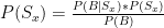
Let’s say “WM” = the odds of the Heat winning the series. So now we need to find EV(iM) in terms of bM and WM. If Ilardi picks Miami, he wins every time I pick Miami, and every time Miami wins when I pick Dallas. Thus his expected value for picking Miami is as follows:

$EV(iM)=1*bM+WM*(1-bM)$

When he picks Dallas, he wins every time I don’t pick Miami, and every time Miami loses when I do:

$EV(iD)=1*(1-bM)+(1-WM)*bM$

Setting these two equations equal to each other, the point of indifference can be expressed as follows:

$1*bM+WM*(1-bM)=1*(1-bM)+(1-WM)*bM$

Solving for bM, we get:

$bM=(1-WM)$

What this tells us is MY equilibrium strategy. In other words, if I pick Miami exactly as often as we expect Miami to lose, it doesn’t matter whether Ilardi picks Miami or Dallas, he will win just as often either way.

Now, to find HIS equilibrium strategy, we repeat the process to find the point where I would be indifferent between picking Miami or Dallas:

$EV(bM)=EV(bD)$

$EV(bM)=MW*(1-iM)$

$EV(bD)=(1-MW)*iM$

$MW*(1-iM)=(1-MW)*iM$

$iM=WM$

In other words, if Ilardi picks Miami exactly as often as they are expected to win, it doesn’t matter which team I pick.

Note the elegance of the solution: Ilardi should pick each team exactly as often as they are expected to win, and I should pick each team exactly as often as they are expected to lose. There are actually a lot of theorems and such that you’d learn in a Game Theory class that make identifying that kind of situation much easier, but I’m pretty rusty on that stuff myself.

So how often would each of us win in the equilibrium solution? To find this, we can just solve any of the EV equations above, substituting the opposing player’s optimal strategy for the variable representing the same. So let’s use the EV(iM) equation, substituting (1-WM) anywhere bM appears:

$EV(iEq)=1*(1-WM)+WM*(1-(1-WM))$

Simplify:

$EV(iEq)=1 - WM +WM^2$

Here’s a graph of the function:

Obviously, it doesn’t matter which team is favored: Ilardi’s edge is weakest when the series is a tossup, where he should win 75% of the time. The bigger a favorite one team is, the bigger the leader’s advantage.

Now let’s Assume Miami was expected to win 63% of the time (approximately the consensus), the Nash Equilibrium strategy would give Ilardi a 76.7% chance of winning, which is obviously considerably better than the 63% chance that he ended up with by choosing Miami to my Dallas—so the actual picks were a favorable outcome for me. Of course, that’s not to say his decision was wrong from his perspective: Either of us could have other preferences that come into play—for example, we might intrinsically value picking the Finals correctly, or someone in my spot (though probably not me) might care more about securing their 2nd-place finish than about having a chance to overtake the leader, or Ilardi might want to avoid looking bad if he “outsmarted himself” by picking Dallas while I played straight-up and stuck with Miami.

But even assuming we both wanted to maximize our chances of winning the competition, picking Miami may still have been Ilardi’s best strategy given when he knew at the time, and it would have been a fairly common outcome if we had both played game-theoretically anyway. Which brings me to the main purpose for this post:

A Little Meta-Strategy

In reality, neither of us played our equilibrium strategies. I believed Ilardi would pick Miami more than 63% of the time, and thus the correct choice for me was to pick Dallas. Assuming Ilardi believed I would pick Dallas less than 63% of the time, his best choice was to pick Miami. Indeed, it might seem almost foolhardy to actually play a mixed strategy: what are the chances that your opponent ever actually makes a certain choice exactly 37% of the time? Whatever your estimation, you should go with whichever gives you the better expected value, right?

This is a conundrum that should be familiar to any serious poker players out there. E.g., at the end of the hand, you will frequently find yourself in an “is he bluffing or not?” (or “should I bluff or not?”) situation. You can work out the game-theoretically optimal calling (or bluffing) rate and then roll a die in your head. But really, what are the chances that your opponent is bluffing exactly the correct percentage of the time? To maximize your expected value, you gauge your opponent’s chances of bluffing, and if you have the correct pot odds, you call or fold (or raise) as appropriate.

So why would you ever play the game-theoretical strategy, rather than just making your best guess about what your opponent is doing and responding to that? There are a couple of answers to this. First, in a repeating game, there can be strategic advantages to having your opponent know (or at least believe) that you are playing such a strategy. But the slightly trickier—and for most people, more important—answer is that your estimation might be wrong: playing the “unexploitable” strategy is a defensive maneuver that ensures your opponent isn’t outsmarting you.

The key is that playing any “exploiting” strategy opens you up to be exploited yourself. Think again of Rock-Paper-Scissors: If you’re pretty sure your opponent is playing “rock” too often, you can try to exploit them by playing “paper” instead of randomizing—but this opens you up for the deadly “scissors” counterattack. And if your opponent is a step ahead of you (or a level above you), he may have anticipated (or even set up) your new strategy, and has already prepared to take advantage.

Though it may be a bit of an oversimplification, I think a good meta-strategy for this kind of situation—where you have an equilibrium or “unexploitable” strategy available, but are tempted to play an exploiting but vulnerable strategy instead—is to step back and ask yourself the following question: For this particular spot, if you get into a leveling contest with your opponent, who is more likely to win? If you believe you are, then, by all means, exploit away. But if you’re unsure about his approach, and there’s a decent chance he may anticipate yours—that is, if he’s more likely to be inside your head than you are to be inside his—your best choice may be to avoid the leveling game altogether. There’s no shame in falling back on the “unexploitable” solution, confident that he can’t possibly gain an advantage on you.

Back in Smackdown-land: Given the consensus view of the series, again, the equilibrium strategy would have given Ilardi about a 77% chance of winning. And he could have announced this strategy to the world—it wouldn’t matter, as there’s nothing I could have done about it. As noted above, when the actual picks came out, his new probability (63%) was significantly lower. Of course, we shouldn’t read too much into this: it’s only a single result, and doesn’t prove that either one of us had an advantage. On the other hand, I did make that pick in part because I felt that Ilardi was unlikely to “outlevel” me. To be clear, this was not based on any specific assessment about Ilardi personally, but based my general beliefs about people’s tendencies in that kind of situation.

Was I right? The outcome and reasoning given in the final “picking game” has given me no reason to believe otherwise, though I think that the reciprocal lack of information this time around was a major part of that advantage. If Ilardi and I find ourselves in a similar spot in the future (perhaps in next year’s Smackdown), I’d guess the considerations on both sides would be quite different.