Graph of the Day: When Do Undefeated Teams Lose?

The Kansas City Chiefs beat Buffalo today to push their record to 9-0, with Alex Smith once again putting up numbers only his mother or Terry Bradshaw could love (too bad he doesn’t have Randy Moss). There has been a lot of grumbling about this Chiefs team, and for a serious-ish treatment see “The Worst 8-0 Team of All Time?” at Advanced NFL Stats.

However, their victory is perfectly consistent with the long and storied history of 8-0 teams, who have a 19-2 record in game 9 (through today). Indeed, of all “x-0” teams (where X is less than 15), 8-0 is the least likely to lose their next game:

undefeated

And if you counted all the remaining games of 15-0 teams, they would still only be 5-1 (the ’72 Dolphins went undefeated, and the 2007 Patriots won 3 more before losing the Super Bowl).

What does this mean? Probably not that much, though late regular-season NFL gets wacky for a number of reasons (injuries, strategic incentives, motivational changes, etc), so it’s unsurprising to me that the “drop rate” increases even as the teams should theoretically be getting stronger.

In bad news for the Chiefs, however, their odds of winning the Super Bowl decreased slightly: while 40% of 8-0 teams had gone on to a championship, only 39% of 9-0 teams have done the same (classic DUCY).

Is Randy Moss the Greatest?

So apparently San Francisco backup wide receiver Randy Moss made some headlines at Super Bowl media day by expressing the opinion that he is the greatest receiver of all time.

Much of the response I’ve seen on Twitter has looked like this:

The ESPN article similarly emphasizes Jerry Rice’s superior numbers:

[Moss] has 982 catches for 15,292 yards and 156 touchdowns in his 14-season career.

Hall of Famer Jerry Rice, who now is an ESPN NFL analyst, leads the all-time lists in those three categories with 1,549 receptions, 22,895 yards and 197 touchdown receptions.

Elsewhere, they do note that Jerry Rice played 20 seasons.

Mike Sando has some analysis and a round-up of analyst and fan reactions, including several similar points under heading “The Stats”, and this slightly snarky caption:

Randy Moss says he’s the greatest WR of all time. @JerryRice: “Put my numbers up against his numbers.” We did –>

So when I first saw this story, I kind of laughed it off (generally I’m against claims of greatness that don’t come with 150-page proofs), but then I saw what Randy Moss actually said:

“I don’t really live on numbers, I really live on impact and what you’re able to do out on the field,” he said Tuesday. “I really think I’m the greatest receiver to ever play this game.”

From this, I think the only logical conclusion is that Randy Moss clearly reads this blog.

As any of my ultra-long-time readers know, I’ve written about Randy Moss before. “Quantum Randy Moss—An Introduction to Entanglement” was one of my earliest posts (and probably my first ever to be read by anyone other than friends and family).

Cliff’s Notes version: I think Moss is right that yards and touchdowns and other production “numbers” don’t matter as much as “impact”, or what a player’s actual affect is on his team’s ability to move the ball, score points, and ultimately win games. Unfortunately, isolating a player’s “true value” can be virtually impossible in the NFL, since everyone’s stats are highly “entangled.” However, Randy Moss may come the closest to having a robust data set that’s actually on point, since, for a variety of reasons, he has played with a LOT of different quarterbacks. When I wrote that article, it was clear that all of them played *much* better with Moss than without him.

Given this latest “controversy,” I thought I’d take a quick chance to update my old data. After all, Tom Brady and Matt Cassell have played some more seasons since I did my original analysis. Also, while it may or may not be relevant given Moss’s more limited role and lower statistical production, Alex Smith now actually qualifies under my original criteria (playing at least 9 games with Randy Moss in a single season). So, for what it’s worth, I’ve included him as well. Here’s the updated comparison of seasons with Randy Moss vs. career without him (for more details, read the original article):

Note: I calculated these numbers a tiny bit differently than before. specifically, I cut out all performance stats from seasons in which a QB didn’t play at least 4 games.

Of course, Alex Smith had a much better season last year than he has previously in his career, so that got me thinking it might be worth trying to make a slightly more apples-to-apples comparison for all 7 quarterbacks. So I filtered the data to compare seasons with Randy Moss only against “Bookend” seasons—that is, each quarterback’s seasons immediately before or after playing with Moss (if applicable):

Here we can see a little bit more variability, as we would expect considering the smaller sample of seasons for comparison, but the bottom line is unchanged. On average, the “Moss effect” even appears to be slightly larger overall. Adjusted Net Yards Per Attempt is probably the best single metric for measuring QB/passing game efficiency, and a difference of 1.77 is about what separates QB’s like Aaron Rodgers from Shaun Hill (7.54 v. 5.68), or a Peyton Manning from a Gus Frerotte (7.11 v. 5.27).

This magnitude of difference is down slightly from the calculations I did in 2010. This is partly because of a change in method (see “note” above), but (in fairness), also partly because Tom Brady’s “non Moss” numbers have improved a bit in the last couple of seasons. On the other hand, the samples are also larger, which makes the unambiguous end result a bit more reliable.

Even Smith clearly still had better statistics this season with Moss (not to mention Colin Kaepearnick seems to be doing OK as well).  Whether that improvement is due to Moss (or more likely, the fear of Moss), who knows. For any particular case(s), there may be/probably are other factors at play: By no means am I saying these are all fair comparisons. But better results in this type of comparison are more likely to occur the better the player actually was. Thus, as a Bayesian matter, extreme results like these make it likely that Randy Moss was extremely good.

So does this mean I think Moss is right? Really, I have no idea. “Greatness” is a subjective term, and Rice clearly had a longer and more fruitful (3 Super Bowl rings) career. But for actual “impact” on the game: If I were a betting man (and I am), I’d say that the quality and strength of evidence in Moss’s favor makes him the most likely “best ever” candidate.

[1/31 Edit: Made some minor clarifying changes throughout.]

Don’t Play Baseball With Bill Belichick

[Note: I apologize for missing last Wednesday and Friday in my posting schedule. I had some important business-y things going on Wed and then went to Canada for a wedding over the weekend.]

Last week I came across this ESPN article (citing this Forbes article) about how Bill Belichick is the highest-paid coach in American sports:

Bill Belichick tops the list for the second year in a row following the retirement of Phil Jackson, the only coach to have ever made an eight-figure salary. Belichick is believed to make $7.5 million per year. Doc Rivers is the highest-paid NBA coach at $7 million.

Congrats to Belichick for a worthy accomplishment! Though I still think it probably under-states his actual value, at least relative to NFL players. As I tweeted:

Of course, coaches’ salaries are different from players’: they aren’t constrained by the salary cap, nor are they boosted by the mandatory revenue-sharing in the players’ collective bargaining agreement.  Yet, for comparison, this season Belichick will make a bit more than a third of what Peyton Manning will in Denver. As I’ve said before, I think Belichick and Manning have been (almost indisputably) the most powerful forces in the modern NFL (maybe ever). Here’s the key visual from my earlier post, updated to include last season (press play):

The x axis is wins in season n, y axis is wins in season n+1.

Naturally, Belichick has benefited from having Tom Brady on his team. However, Brady makes about twice as much as Belichick does, and I think you would be hard-pressed to argue that he’s twice as valuable—and I think top QB’s are probably underpaid relative to their value anyway.

But being high on Bill Belichick is about more than just his results. He is well-loved in the analytical community, particularly for some of his high-profile 4th down and other in-game tactical decisions.  But I think those flashy calls are merely a symptom of his broader commitment to making intelligent win-maximizing decisions—a commitment that is probably even more evident in the decisions he has made and strategies he has pursued in his role as the Patriots’ General Manager.

But rather than sorting through everything Belichick has done that I like, I want to take a quick look at one recent adjustment that really impressed me: the Patriots out-of-character machinations in the 2012 draft.

The New Rookie Salary Structure

One of the unheralded elements to the Patriots’ success—perhaps rivaling Tom Brady himself in actual importance—is their penchant for stock-piling draft-picks in the “sweet spot” of the NFL draft (late 1st to mid-2nd round), where picks have the most surplus value. Once again, here’s the killer graph from the famous Massey-Thaler study on the topic:

In the 11 drafts since Belichick took over, the Patriots have made 17 picks between numbers 20 and 50 overall, the most in the NFL (the next-most is SF with 15, league average is obv 11). To illustrate how unusual their draft strategy has been, here’s a plot of their 2nd round draft position vs. their total wins over the same period:

Despite New England having the highest win percentage (not to mention most Super Bowl wins and appearances) over the period, there are 15 teams with lower average draft positions in the 2nd round. For comparison, they have the 2nd lowest average draft position in the 1st round and 7th lowest in the third.

Of course, the new collective bargaining agreement includes a rookie salary scale. Without going into all the details (in part because they’re extremely complicated and not entirely public), the key points are that it keeps total rookie compensation relatively stable while flattening the scale at the top, reducing guaranteed money, and shortening the maximum number of years for each deal.

These changes should all theoretically flatten out the “value curve” above. Here’s a rough sketch of what the changes seem to be attempting:

Since the original study was published, the dollar values have gone up and the top end has gotten more skewed. I adjusted the Y-axis to reflect the new top, but didn’t adjust the curve itself, so it should actually be somewhat steeper than it appears.  I tried to make the new curves as conceptually accurate as I could, but they’re not empirical and should be considered more of an “artist’s rendition” of what I think the NFL is aiming for.

With a couple of years of data, this should be a very interesting issue to revisit.  But, for now, I think it’s unlikely that the curve will actually be flattened very much. If I had to guess, I think it may end up “dual-peaked”: By far the greatest drop in guaranteed money will be for top QB prospects taken with the first few picks. These players already provide the most value, and are the main reason the original M/T performance graph inclines so steeply on the left. Additionally, they provide an opportunity for continued surplus value beyond the length of the initial contract. This should make the top of the draft extremely attractive, at least in years with top QB prospects.

On the other hand, I think the bulk of the effect on the rest of the surplus-value curve will be to shift it to the left. My reasons for thinking this are much more complicated, and include my belief that the original Massey/Thaler study has problems with its valuation model, but the extremely short version is that I have reason to believe that people systematically overvalue upper/middle 1st round picks.

How the Patriots Responded

Since I’ve been following the Patriots’ 2nd-round-oriented drafting strategy for years now, naturally my first thoughts after seeing the details of the new deal went to how this could kill their edge. Here’s a question I tweeted at the Sloan conference:

Actually, my concern about the Patriots drafting strategy was two-fold:

  1. The Patriots favorite place to draft could obviously lose its comparative value under the new system. If they left their strategy as-is, it could lead to their picking sub-optimally. At the very least, it should eliminate their exploitation opportunity.
  2. Though a secondary issue for this post, at some point  taking an extreme bang-for-your-buck approach to player value can run into diminishing returns and cause stagnation. Since you can only have so many players on your roster or on the field at a time, your ability to hoard and exploit “cheap” talent is constrained. This is a particularly big concern for teams that are already pretty good, especially if they already have good “value” players in a lot of positions: At some point, you need players who are less cheap but higher quality, even if their value per dollar is lower than the alternative.

Of course, if you followed the draft, you know that the Patriots, entering the draft with far fewer picks than usual, still traded up in the 1st round, twice.

Taken out of context, these moves seem extremely out of character for the Patriots. Yet the moves are perfectly consistent with an approach that understands and attacks my concerns: Making fewer, higher-quality picks is essentially the correct solution, and if the value-curve has indeed shifted up as I expect it has, the new epicenter of the Patriots’ draft activity may be directly on top of the new sweet spot.

Baseball

The entire affair reminds me of an old piece of poker wisdom that goes something like this: In a mixed game with one truly expert poker player and a bunch of completely outclassed amateurs, the expert’s biggest edge wouldn’t come in the poker variant with which he has the most expertise, but in some ridiculous spontaneous variant with tons of complicated made-up rules.

I forget where I first read the concept, but I know it has been addressed in various ways by many authors, ranging from Mike Caro to David Sklansky. I believe it was the latter (though please correct me if I’m wrong), who specifically suggested a Stud variant some of us remember fondly from childhood:

Several different games played only in low-stakes home games are called Baseball, and generally involve many wild cards (often 3s and 9s), paying the pot for wild cards, being dealt an extra upcard upon receiving a 4, and many other ad-hoc rules (for example, the appearance of the queen of spades is called a “rainout” and ends the hand, or that either red 7 dealt face-up is a rainout, but if one player has both red 7s in the hole, that outranks everything, even a 5 of a kind). These same rules can be applied to no peek, in which case the game is called “night baseball”.

The main ideas are that A) the expert would be able to adapt to the new rules much more quickly, and B) all those complicated rules make it much more likely that he would be able to find profitable exploitations (for Baseball in particular, there’s the added virtue of having several betting rounds per hand).

It will take a while to see how this plays out, and of course the abnormal outcome could just be a circumstances-driven coincidence rather than an explicit shift in the Patriots’ approach. But if my intuitions about the situation are right, Belichick may deserve extra credit for making deft adjustments in a changing landscape, much as you would expect from the Baseball-playing shark.

Sports Geek Mecca: Recap and Thoughts, Part 2

This is part 2 of my “recap” of the Sloan Sports Analytics Conference that I attended in March (part 1 is here), mostly covering Day 2 of the event, but also featuring my petty way-too-long rant about Bill James (which I’ve moved to the end).

Day Two

First I attended the Football Analytics despite finding it disappointing last year, and, alas, it wasn’t any better. Eric Mangini must be the only former NFL coach willing to attend, b/c they keep bringing him back:

Overall, I spent more time in day 2 going to niche panels, research paper presentations and talking to people.

The last, in particular, was great. For example, I had a fun conversation with Henry Abbott about Kobe Bryant’s lack of “clutch.” This is one of Abbott’s pet issues, and I admit he makes a good case, particularly that the Lakers are net losers in “clutch” situations (yes, relative to other teams), even over the periods where they have been dominant otherwise.

Kobe is kind of a pivotal case in analytics, I think. First, I’m a big believer in “Count the Rings, Son” analysis: That is, leading a team to multiple championships is really hard, and only really great players do it. I also think he stands at a kind of nexus, in that stats like PER give spray shooters like him an unfair advantage, but more finely tuned advanced metrics probably over-punish the same. Part of the burden of Kobe’s role is that he has to take a lot of bad shots—the relevant question is how good he is at his job.

Abbott also mentioned that he liked one of my tweets, but didn’t know if he could retweet the non-family-friendly “WTF”:

I also had a fun conversation with Neil Paine of Basketball Reference. He seemed like a very smart guy, but this may be attributable to the fact that we seemed to be on the same page about so many things. Additionally, we discussed a very fun hypo: How far back in time would you have to go for the Charlotte Bobcats to be the odds-on favorites to win the NBA Championship?

As for the “sideshow” panels, they’re generally more fruitful and interesting than the ESPN-moderated super-panels, but they offer fewer easy targets for easy blog-griping. If you’re really interested in what went down, there is a ton of info at the SSAC website. The agenda can be found here. Information on the speakers is here. And, most importantly, videos of the various panels can be found here.

Box Score Rebooted

Featuring Dean Oliver, Bill James, and others.

This was a somewhat interesting, though I think slightly off-target, panel. They spent a lot of time talking about new data and metrics and pooh-poohing things like RBI (and even OPS), and the brave new world of play-by-play and video tracking, etc. But too much of this was discussing a different granularity of data than what can be improved in the current granularity levels. Or, in other words:

James acquitted himself a bit on this subject, arguing that boatloads of new data isn’t useful if it isn’t boiled down into useful metrics. But a more general way of looking at this is: If we were starting over from scratch, with a box-score-sized space to report a statistical game summary, and a similar degree of game-scoring resources, what kinds of things would we want to include (or not) that are different from what we have now?  I can think of a few:

  1. In basketball, it’s archaic that free-throws aren’t broken down into bonus free throws and shot-replacing free throws.
  2. In football, I’d like to see passing stats by down and distance, or at least in a few key categories like 3rd and long.
  3. In baseball, I’d like to see “runs relative to par” for pitchers (though this can be computed easily enough from existing box scores).

In this panel, Dean Oliver took the opportunity to plug ESPN’s bizarre proprietary Total Quarterback Rating. They actually had another panel devoted just to this topic, but I didn’t go, so I’ll put a couple of thoughts here.

First, I don’t understand why ESPN is pushing this as a proprietary stat. Sure, no-one knows how to calculate regular old-fashioned quarterback ratings, but there’s a certain comfort in at least knowing it’s a real thing. It’s a bit like Terms of Service agreements, which people regularly sign without reading: at least you know the terms are out there, so someone actually cares enough to read them, and presumably they would raise a stink if you had to sign away your soul.

As for what we do know, I may write more on this come football season, but I have a couple of problems:

One, I hate the “clutch effect.” TQBR makes a special adjustment to value clutch performance even more than its generic contribution to winning. If anything, clutch situations in football are so bizarre that they should count less. In fact, when I’ve done NFL analysis, I’ve often just cut the 4th quarter entirely, and I’ve found I get better results. That may sound crazy, but it’s a bit like how some very advanced Soccer analysts have cut goal-scoring from their models, instead just focusing on how well a player advances the ball toward his goal: even if the former matters more, its unreliability may make it less useful.

Two, I’m disappointed in the way they “assign credit” for play outcomes:

Division of credit is the next step. Dividing credit among teammates is one of the most difficult but important aspects of sports. Teammates rely upon each other and, as the cliché goes, a team might not be the sum of its parts. By dividing credit, we are forcing the parts to sum up to the team, understanding the limitations but knowing that it is the best way statistically for the rating.

I’m personally very interested in this topic (and have discussed it with various ESPN analytics guys since long before TQBR was released). This is basically an attempt to address the entanglement problem that permeates football statistics.  ESPN’s published explanation is pretty cryptic, and it didn’t seem clear to me whether they were profiling individual players and situations or had created credit-distribution algorithms league-wide.

At the conference, I had a chance to talk with their analytics guy who designed this part of the metric (his name escapes me), and I confirmed that they modeled credit distribution for the entire league and are applying it in a blanket way.  Technically, I guess this is a step in the right direction, but it’s purely a reduction of noise and doesn’t address the real issue.  What I’d really like to see is like a recursive model that imputes how much credit various players deserve broadly, then uses those numbers to re-assign credit for particular outcomes (rinse and repeat).

Deconstructing the Rebound With Optical Tracking Data

Rajiv Maheswaran, and other nerds.

This presentation was so awesome that I offered them a hedge bet for the “Best Research Paper” award. That is, I would bet on them at even money, so that if they lost, at least they would receive a consolation prize. They declined. And won. Their findings are too numerous and interesting to list, so you should really check it out for yourself.

Obviously my work on the Dennis Rodman mystery makes me particularly interested in their theories of why certain players get more rebounds than others, as I tweeted in this insta-hypothesis:

Following the presentation, I got the chance to talk with Rajiv for quite a while, which was amazing. Obviously they don’t have any data on Dennis Rodman directly, but Rajiv was also interested in him and had watched a lot of Rodman video. Though anecdotal, he did say that his observations somewhat confirmed the theory that a big part of Rodman’s rebounding advantage seemed to come from handling space very well:

  1. Even when away from the basket, Rodman typically moved to the open space immediately following a shot. This is a bit different from how people often think about rebounding as aggressively attacking the ball (or as being able to near-psychically predict where the ball is going to come down.
  2. Also rather than simply attacking the board directly, Rodman’s first inclination was to insert himself between the nearest opponent and the basket. In theory, this might slightly decrease the chances of getting the ball when it heads in toward his previous position, but would make up for it by dramatically increasing his chances of getting the ball when it went toward the other guy.
  3. Though a little less purely strategical, Rajiv also thought that Rodman was just incredibly good at #2. That is, he was just exceptionally good at jockeying for position.

To some extent, I guess this is just rebounding fundamentals, but I still think it’s very interesting to think about the indirect probabilistic side of the rebounding game.

Live B.S. Report with Bill James

Quick tangent: At one point, I thought Neil Paine summed me up pretty well as a “contrarian to the contrarians.”  Of course, I’m don’t think I’m contrary for the sake of contrariness, or that I’m a negative person (I don’t know how many times I’ve explained to my wife that just because I hated a movie doesn’t mean I didn’t enjoy it!), it’s just that my mind is naturally inclined toward considering the limitations of whatever is put in front of it. Sometimes that means criticizing the status quo, and sometimes that means criticizing its critics.

So, with that in mind, I thought Bill James’s showing at the conference was pretty disappointing, particularly his interview with Bill Simmons.

I have a lot of respect for James.  I read his Historical Baseball Abstract and enjoyed it considerably more than Moneyball.  He has a very intuitive and logical mind. He doesn’t say a bunch of shit that’s not true, and he sees beyond the obvious. In Saturday’s “Rebooting the Box-score” panel, he made an observation that having 3 of 5 people on the panel named John implied that the panel was [likely] older than the rest of the room.  This got a nice laugh from the attendees, but I don’t think he was kidding.  And whether he was or not, he still gets 10 kudos from me for making the closest thing to a Bayesian argument I heard all weekend.  And I dutifully snuck in for a pic with him:

James was somewhat ahead of his time, and perhaps he’s still one of the better sports analytic minds out there, but in this interview we didn’t really get to hear him analyze anything, you know, sportsy. This interview was all about Bill James and his bio and how awesome he was and how great he is and how hard it was for him to get recognized and how much he has changed the game and how, without him, the world would be a cold, dark place where ignorance reigned and nobody had ever heard of “win maximization.”

Bill Simmons going this route in a podcast interview doesn’t surprise me: his audience is obviously much broader than the geeks in the room, and Simmons knows his audience’s expectations better than anyone. What got to me was James’s willingness to play along, and everyone else’s willingness to eat it up. Here’s an example of both, from the conference’s official Twitter account:

Perhaps it’s because I never really liked baseball, and I didn’t really know anyone did any of this stuff until recently, but I’m pretty certain that Bill James had virtually zero impact on my own development as a sports data-cruncher.  When I made my first PRABS-style basketball formula in the early 1990’s (which was absolutely terrible, but is still more predictive than PER), I had no idea that any sports stats other than the box score even existed. By the time I first heard the word “sabermetrics,” I was deep into my own research, and didn’t bother really looking into it deeply until maybe a few months ago.

Which is not to say I had no guidance or inspiration.  For me, a big epiphanous turning point in my approach to the analysis of games did take place—after I read David Sklansky’s Theory of Poker. While ToP itself was published in 1994, Sklansky’s similar offerings date back to the 70s, so I don’t think any broader causal pictures are possible.

More broadly, I think the claim that sports analytics wouldn’t have developed without Bill James is preposterous. Especially if, as i assume we do, we firmly believe we’re right.  This isn’t like L. Ron Hubbard and Incident II: being for sports analytics isn’t like having faith in a person or his religion. It simply means trying to think more rigorously about sports, and using all of the available analytical techniques we can to gain an advantage. Eventually, those who embrace the right will win out, as we’ve seen begin to happen in sports, and as has already happened in nearly every other discipline.

Indeed, by his own admission, James liked to stir controversy, piss people off, and talk down to the old guard whenever possible. As far as we know, he may have set the cause of sports analytics back, either by alienating the people who could have helped it gain acceptance, or by setting an arrogant and confrontational tone for his disciples (e.g., the uplifting “don’t feel the need to explain yourself” message in Moneyball). I’m not saying that this is the case or even a likely possibility, I’m just trying to illustrate that giving someone credit for all that follows—even a pioneer like James—is a dicey game that I’d rather not participate in, and that he definitely shouldn’t.

On a more technical note, one of his oft-quoted and re-tweeted pearls of wisdom goes as follows:

Sounds great, right? I mean, not really, I don’t get the metaphor: if the sea is full of ignorance, why are you collecting water from it with a bucket rather than some kind of filtration system? But more importantly, his argument in defense of this claim is amazingly weak. When Simmons asked what kinds of things he’s talking about, he repeatedly emphasized that we have no idea whether a college sophomore will turn out to be a great Major League pitcher.  True, but, um, we never will. There are too many variables, the input and outputs are too far apart in time, and the contexts are too different.  This isn’t the sea of ignorance, it’s a sea of unknowns.

Which gets at one of my big complaints about stats-types generally.  A lot of people seem to think that stats are all about making exciting discoveries and answering questions that were previously unanswerable. Yes, sometimes you get lucky and uncover some relationship that leads to a killer new strategy or to some game-altering new dynamic. But most of the time, you’ll find static. A good statistical thinker doesn’t try to reject the static, but tries to understand it: Figuring out what you can’t know is just as important as figuring out what you can know.

On Twitter I used this analogy:

Success comes with knowing more true things and fewer false things than the other guy.

Championship Experience Matters! (Super Bowl Edition)

To complete “Championship Week” at Skeptical Sports, I thought I’d post a little fun research I did before this year’s Super Bowl.

Like basketball, teams with championship-winning experience outperform their regular-season records in the playoffs, especially if they make it to the Super Bowl.

So, a bit like my 5-by-5 model, I wanted to come up with a simple metric for picking the Super Bowl winner. Unlike its NBA cousin, however, this method only applies to the championship game, not to the entire playoffs. The main question is, how much better does a team with more Super Bowl winning experience do than it’s opponent?

I feel bad about my text/graphs ratio this week, so I thought I’d tell this story in pictures. Before testing the question, we need to pick the best time period. So, for what number of years does the metric “pick the team with the most super bowl wins” most often pick the ultimate winner:

This was a little surprising to me already: I thought for sure the best n would be a small number, but it turns out to be 6.

Counting 2012, there have been 26 Super Bowls where one team has won more championships in the previous 6 years than the other. Of those games, the team with the greater number has won 20, or 77% of the time—including the Giants. [True story: I was going to publish something on this research before this year’s Super Bowl, but, knowing that it predicted a New York win against the heavily favored Patriots, I chickened out.]

Of course, I’m sure most of you are just itching to pounce right now: Clearly the team with the most recent Super Bowl wins is usually going to be better, right? So clearly this must be confounding this result. So let’s compare it to the predictive accuracy of SRS (Simple Rating System, aka “Margin of Victory adjusted for Strength of Schedule”):

Looking at all 46 Super Bowls, the team with the higher SRS has won 26, or 57%. In Super Bowls where no team had more Super Bowl wins, SRS performs slightly better, correctly picking 12/20 (60%). But the real story is in the games where both had something to say: When SRS and L6 agreed, the team they both picked won 11/14 (79%). But when SRS and L6 disagreed—in other words, where one team had a higher SRS, but the other had more Super Bowl wins in the previous 6 years—the team with the paper qualifications lost to the team with the championship experience 9 of 12 times (75%).

Now, your next thought might be that the years when L6 trumped SRS were probably the years when the teams were very close. But you’d be wrong:

The average SRS difference in 9 years where the L6 team won is actually higher than in the 3 years when it lost!

So how much does L6 add overall? Well, let’s first create a simple method, a bit like 5-by-5:

  1. If one team has more Super Bowl wins in the previous 6 years, pick them.
  2. Otherwise, pick the team with the best SRS.

Following this method, you would correctly pick 32 of the 46 Super Bowls (70%), for a 10% improvement overall, despite step 1 only even applying in about half of the games (also, note that if you just picked randomly in the 20 Super Bowls where L6 doesn’t apply, you would still be expected to get 30 right overall).

Finally, to try to quantify the difference in predictive value between the two measures, I plugged them both into a logistic regression:

As you can see, L6 is much more predictive, though the 95% confidence intervals do overlap. (Though I should also note, this last chart is based on the regression I ran prior to this year’s game, which ended up being another victory for the championship experience side.)

Graph of the Day: Quarterbacks v. Coaches, Draft Edition

[Note: With the recent amazing addition to my office, I’ve considered just turning this site into a full-on baby photo-blog (much like my Twitter feed).  While that would probably mean a more steady stream of content, it would also probably require a new name, a re-design, and massive structural changes.  Which, in turn, would raise a whole bevy of ontological issues that I’m too tired to deal with at the moment. So I guess back to sports analysis!]

In “A History of Hall of Fame QB-Coach Entanglement,” I talked a bit about the difficulty of “detangling” QB and coach accomplishments.  For a slightly more amusing historical take, here’s a graph illustrating how first round draft picks have gotten a much better return on investment (a full order of magnitude better vs. non-#1 overalls) when traded for head coaches than when used to draft quarterbacks:

Note: Since 1950. List of #1 Overall QB’s is here.  Other 1st Round QB’s here.  Other drafted QB’s here.  Super Bowl starters here.  QB’s that were immediately traded count for the team that got them.

Note*: . . that I know of. I googled around looking for coaches that cost their teams at least one first round draft pick to acquire, and I could only find 3: Bill Parcells (Patriots -> Jets), Bill Belichick (Jets -> Patriots), and Jon Gruden (Raiders -> Bucs).  If I’m missing anyone, please let me know.

Sample, schmample.

But seriously, the other 3 bars are interesting too.

Thoughts on the Packers Yardage Anomaly

In their win over Detroit on Sunday, Green Bay once again managed to emerge victorious despite giving up more yards than they gained. This is practically old hat for them, as it’s the 10th time that they’ve done it this year. Over the course of the season, the 15-1 Packers gave up a stunning 6585 yards, while gaining “just” 6482—thus losing the yardage battle despite being the league’s most dominant team.

This anomaly certainly captures the imagination, and I’ve received multiple requests for comment.  E.g., a friend from my old poker game emails:

Just heard that the Packers have given up more yards than they’ve gained and was wondering how to explain this.  Obviously the Packers’ defense is going to be underrated by Yards Per Game metrics since they get big leads and score quickly yada yada, but I don’t see how this has anything to do with the fact they’re being outgained.  I assume they get better starting field position by a significant amount relative to their opponents so they can have more scoring drives than their opponents while still giving up more yards than they gain, but is that backed up by the stats?

Last week Advanced NFL Stats posted a link to this article from Smart Football looking into the issue in a bit more depth. That author does a good job examining what this stat means, and whether or not it implies that Green Bay isn’t as good as they seem (he more or less concludes that it doesn’t).

But that doesn’t really answer the question of how the anomaly is even possible, much less how or why it came to be.  With that in mind, I set out to solve the problem.  Unfortunately, after having looked at the issue from a number of angles, and having let it marinate in my head for a week, I simply haven’t found an answer that I find satisfying.  But, what the hell, one of my resolutions is to pull the trigger on this sort of thing, so I figure I should post what I’ve got.

How Anomalous?

The first thing to do when you come across something that seems “crazy on its face” is to investigate how crazy it actually is (frequently the best explanation for something unusual is that it needs no explanation).  In this case, however, I think the Packers’ yardage anomaly is, indeed, “pretty crazy.”  Not otherworldly crazy, but, say, on a scale of 1 to “Kurt Warner being the 2000 MVP,” it’s at least a 6.

First, I was surprised to discover that just last year, the New England Patriots also had the league’s best record (14-2), and also managed to lose the yardage battle.  But despite such a recent example of a similar anomaly, it is still statistically pretty extreme.  Here’s a plot of more or less every NFL team season from 1936 through the present, excluding seasons where the relevant stats weren’t available or were too incomplete to be useful (N=1647):

The green diamond is the Packers net yardage vs. Win%, and the yellow triangle is their net yardage vs. Margin of Victory (net points).  While not exactly Rodman-esque outliers, these do turn out to be very historically unusual:

Win %

Using the trendline equation on the graph above (plus basic algebra), we can use a team’s season Win percentage to calculate their expected yardage differential.  With that prediction in hand, we can compare how much each team over or under-performed its “expectation”:

Both the 2011 Packers and the 2010 Patriots are in the top 5 all-time, and I should note that the 1939 New York Giants disparity is slightly overstated, because I excluded tie games entirely (ties cause problems elsewhere b/c of perfect correlation with MOV).

Margin of Victory

Toward the conclusion of that Smart Football article, the author notes that Green Bay’s Margin of Victory isn’t as strong as their overall record, noting that the Packers “Pythagorian Record” (expectation computed from points scored and points allowed) is more like 11-5 or 12-4 than 15-1 (note that getting from extremely high Win % to very high MOV is incidental: 15-win teams are usually 11 or 12 win teams that have experienced good fortune).  Green Bay’s MOV of 12.5 is a bit lower than the historical average for 15-1 teams (13.8) but don’t let this mislead you: the disparity between the yardage differential that we would expect based on Green Bay’s MOV and their actual result (using a linear projection, as above) is every bit as extreme as what we saw from Win %:

And here, in histogram form:

So, while not the most unusual thing to ever happen in sports, this anomaly is certainly unusual enough to look into.

For the record, the Packers’ MOV -> yard diff error is 3.23 standard deviations above the mean, while the Win% -> yard diff is 3.28.  But since MOV correlates more strongly with the target stat (note an average error of only 125 yards instead of 170), a similar degree of abnormality leaves it as the more stable and useful metric to look at.

Thus, the problem can be framed as follows: The 2011 Packers fell around 2000 yards (the 125.7 above * 16 games) short of their expected yardage differential.  Where did that 2000 yard gap come from?

Possible Factors and/or Explanations

Before getting started, I should note that, out of necessity, some of these “explanations” are more descriptive than actually explanatory, and even the ones that seem plausible and significant are hopelessly mixed up with one another.  At the end of the day, I think the question of “What happened?” is addressable, though still somewhat unclear.  The question of “Why did it happen?” remains largely a mystery: The most substantial claim that I’m willing to make with any confidence is that none of the obvious possibilities are sufficient explanations by themselves.

While I’m somewhat disappointed with this outcome, it makes sense in a kind of Fermi Paradox, “Why Aren’t They Here Yet?” kind of way.  I.e., if any of the straightforward explanations (e.g., that their stats were skewed by turnovers or “garbage time” distortions) could actually create an anomaly of this magnitude, we’d expect it to have happened more often.

And indeed, the data is actually consistent with a number of different factors (granted, with significant overlap) being present at once.

Line of Scrimmage, and Friends

As suggested in the email above, one theoretical explanation for the anomaly could be the Packers’ presumably superior field position advantage.  I.e., with their offense facing comparatively shorter fields than their opponents, they could have literally had fewer yards available to gain.  This is an interesting idea, but it turns out to be kind of a bust.

The Packers did enjoy a reciprocal field position advantage of about 5 yards.  But, unfortunately, there doesn’t seem to be a noticeable relationship between average starting field position and average yards gained per drive (which would have to be true ex ante for this “explanation” to have any meaning):

Note: Data is from the Football Outsiders drive stats.

This graph plots both offenses and defenses from 2011.  I didn’t look at more historical data, but it’s not really necessary: Even if a larger dataset revealed a statistically significant relationship, the large error rate (which converges quickly) means that it couldn’t alter expectation in an individual case by more than a fraction of a yard or so per possession.  Since Green Bay only traded 175ish possessions this season, it couldn’t even make a dent in our 2000 missing yards (again, that’s if it existed at all).

On the other hand, one thing in the F.O. drive stats that almost certainly IS a factor, is that the Packers had a net of 10 fewer possessions this season than their opponents.  As Green Bay averaged 39.5 yards per possession, this difference alone could account for around 400 yards, or about 20% of what we’re looking for.

Moreover, 5 of those 10 possessions come from a disparity in “zero yard touchdowns,” or net touchdowns scored by their defense and special teams: The Packers scored 7 of these (5 from turnovers, 2 from returns) while only allowing 2 (one fumble recovery and one punt return).  Such scores widen a team’s MOV without affecting their total yardage gap.

[Warning: this next point is a bit abstract, so feel free to skip to the end.] Logically, however, this doesn’t quite get us where we want to go.  The relevant question is “What would the yardage differential have been if the Packers had the same number of possessions as their opponents?”  Some percentage of our 10 counterfactual drives would result in touchdowns regardless.  Now, the Packers scored touchdowns on 37% of their actual drives, but scored touchdowns on at least 50% of their counterfactual drives (the ones that we can actually account for via the “zero yard touchdown” differential).  Since touchdown drives are, on average, longer than non-touchdown drives, this means that the ~400 yards that can be attributed to the possession gap is at least somewhat understated.

Garbage Time

When considering this issue, probably the first thing that springs to minds is that the Packers have won a lot of games easily.  It seems highly plausible that, having rushed out to so many big leads, the Packers must have played a huge amount of “garbage time,” in which their defense could have given up a lot of “meaningless” yards that had no real consequence other than to confound statisticians.

The proportion of yards on each side of the ball that came after Packers games got out of hand should be empirically checkable—but, unfortunately, I haven’t added 2011 Play-by-Play data to my database yet.  That’s okay, though, because there are other ways—perhaps even more interesting ways—to attack the problem.

In fact, it’s pretty much right up my alley: Essentially, what we are looking for here is yet another permutation of “Reverse Clutch” (first discussed in my Rodman series, elaborated in “Tim Tebow and the Taxonomy of Clutch”). Playing soft in garbage time is a great way for a team to “underperform” in statistical proxies for true strength.  In football, there are even a number of sound tactical and strategic reasons why you should explicitly sacrifice yards in order to maximize your chances of winning.  For example, if you have a late lead, you should be more willing to soften up your defense of non-sideline runs and short passes—even if it means giving up more yards on average than a conventional defense would—since those types of plays hasten the end of the game.  And the converse is true on offense:  With a late lead, you want to run plays that avoid turnovers and keep the clock moving, even if it means you’ll be more predictable and easier to defend.

So how might we expect this scenario to play out statistically?  Recall, by definition, “clutch” and “reverse clutch” look the same in a stat sheet.  So what kind of stats—or relationships between stats—normally indicate “clutchness”?  As it turns out, Brian Burke at Advanced NFL Stats has two metrics pretty much at the core of everything he does: Expected Points Added, and Win Percentage Added.  The first of these (EPA) takes the down and distance before and after each play and uses historical empirical data to model how much that result normally affects a team’s point differential.  WPA adds time and score to the equation, and attempts to model the impact each play has on the team’s chances of winning.

A team with “clutch” results—whether by design or by chance—might be expected to perform better in WPA (which ultimately just adds up to their number of wins) than in EPA (which basically measures generic efficiency).

For most aspects of the game, the relationship between these two is strong enough to make such comparisons possible.  Here are plots of this comparison for each of the 4 major categories (2011 NFL, Green Bay in green), starting with passing offense (note that the comparison is technically between wins added overall and expected points per play):

And here’s passing defense:

Rushing offense:

And rushing defense:

Obviously there’s nothing strikingly abnormal about Green Bay’s results in these graphs, but there are small deviations that are perfectly consistent with the garbage time/reverse clutch theory.  For the passing game (offense and defense), Green Bay seems to hew pretty close to expectation.  But in the rushing game they do have small but noticeable disparities on both sides of the ball.  Note that in the scenario I described where a team intentionally trades efficiency for win potential, we would expect the difference to be most acute in the running game (which would be under-defended on defense and overused on offense).

Specifically: Green Bay’s offensive running game has a WPA of 1.1, despite having an EPA per play of zero (which corresponds to a WPA of .25).  On defense, the Packers’ EPA/p is .07, which should correspond to an expected WPA of 1.0, while their actual result is .59.

Clearly, both of these effects are small, considering there isn’t a perfect correlation.  But before dismissing them entirely, I should note that we don’t immediately know how much of the variation in the graphs above is due to variance for a given team and how much is due to variation between teams.  Moreover, without knowing the balance, the fact that both variance and variation contribute to the “entropy” of the observed relationship between EPA/p and WPA, the actual relationship between the two is likely to be stronger than these graphs would make it seem.

The other potential problem is that this comparison is between wins and points, while the broader question is comparing points to yards.  But there’s one other statistical angle that helps bridge the two, while supporting the speculated scenario to boot: Green Bay gained 3.9 yards per attempt on offense, and allowed 4.7 yards per attempt on defense—while the league average is 4.3 yards per attempt.  So, at least in terms of raw yardage, Green Bay performed “below average” in the running game by about .4 yards/attempt on each side of the ball.  Yet, the combined WPA for the Packers running game is positive! Their net rushing WPA is +.5, despite having an expected combined WPA (actually based on their EPA) of -.75.

So, if we thought this wasn’t a statistical artifact, there would be two obvious possible explanations: 1) That Green Bay has a sub-par running game that has happened to be very effective in important spots, or 2) that Green Bay actually has an average (or better) running game that has appeared ineffective (especially as measured by yards gained/allowed) in less important spots. Q.E.D.

For the sake of this analysis, let’s assume that the observed difference for Green Bay here really is a product of strategic adjustments stemming from (or at least related to) their winning ways, how much of our 2000 yard disparity could it account for?

So let’s try a crazy, wildly speculative, back-of-the-envelope calculation: Give Green Bay and its opponents the same number of rushing attempts that they had this season, but with both sides gaining an average number of yards per attempt.  The Packers had 395 attempts and their opponents had 383, so at .4 yards each, the yardage differential would swing by 311 yards.  So again, interesting and plausibly significant, but doesn’t even come close to explaining our anomaly on its own.

Turnover Effect?

One of the more notable features of the Packers season is their incredible +22 turnover margin.  How they managed that and whether it was simply variance or something more meaningful could be its own issue.  But in this context, give them the +22, how helpful is that as an explanation for the yardage disparity?  Turnovers affect scores and outcomes a ton, but are relatively neutral w/r/t yards, so surely this margin is relevant.  But exactly how much does it neutralize the problem?

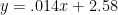
Here, again, we can look at the historical data.  To predict yardage differential based on MOV and turnover differential, we can set up an extremely basic linear regression:

The R-Square value of .725 means that this model is pretty accurate (MOV alone achieved around .66).  Both variables are extremely significant (from p value, or absolute value of t-stat).  Based on these coefficients, the resulting predictive equation is

YardsDiff = 7.84*MOV – 23.3*TOdiff/gm

Running the dataset through the same process as above (comparing predictions with actual results and calculating the total error), here’s how the new rankings turns out:

In other words, if we account for turnovers in our predictions, the expected/actual yardage discrepancy drops from ~125 to ~70 yards per game.  This obv makes the results somewhat less extreme, though still pretty significant: 11th of 1647.  Or, in histogram form:

So what’s the bottom line?  At 69.5 yards per game, the total “missing” yardage drops to around 1100.  Therefore, inasmuch as we accept it as an “explanation,” Green Bay’s turnover differential seems to account for about 900 yards.

It’s probably obvious, but important enough to say anyway, that there is extensive overlap between this “explanation” and our others above: E.g., the interception differential contributes to the possession differential, and is exacerbated by garbage time strategy, which causes the EPA/WPA differential, etc.

“Bend But Don’t Break”

Finally, I have to address a potential cause of this anomaly that I would almost rather not: The elusive “Bend But Don’t Break” defense.  It’s a bit like the Dark Matter of this scenario: I can prove it exists, and estimate about how much is there, but that doesn’t mean I have any idea what it is or where it comes from, and it’s almost certainly not as sexy as people think it is.

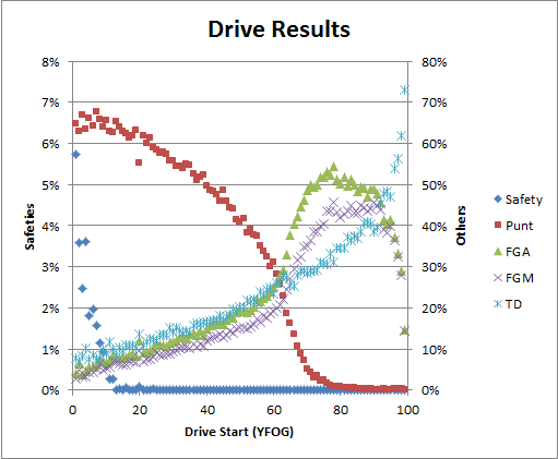
Typically, “Bend But Don’t Break” is the description that NFL analysts use for bad defenses that get lucky.  As a logical and empirical matter, they mostly don’t make sense: Pretty much every team in history (save, possibly, the 2007 New England Patriots) has a steeply inclined expected points by field position curve.  See, e.g., the “Drive Results” chart in this post.  Any time you “bend” enough to give up first downs, you’re giving up expected points. In other words, barring special circumstances, there is simply no way to trade significant yards for a decreased chance of scoring.

Of course, you can have defenses that are stronger at defending various parts of the field, or certain down/distance combinations, which could have the net effect of allowing fewer points than you would expect based on yards allowed, but that’s not some magical defensive rope-a-dope strategy, it’s just being better at some things than others.

But for whatever reason, on a drive-by-drive basis, did the Green Bay defense “bend” more than it “broke”? In other words, did they give up fewer points than expected?

And the answer is “yes.”  Which should be unsurprising, since it’s basically a minor variant of the original problem.  In other words, it begs the question.

In fact, with everything that we’ve looked at so far, this is pretty much all that is left: if there weren’t a significant “Bend But Don’t Break” effect observable, the yardage anomaly would be literally impossible.

And, in fact, this observation “accounts” for about 650 yards, which, combined with everything else we’ve looked at (and assuming a modest amount of overlap), puts us in the ballpark of our initial 2000 yard discrepancy.

Extremely Speculative Conclusions

Some of the things that seem speculative above must be true, because there has to be an accounting: even if it’s completely random, dumb luck with no special properties and no elements of design, there still has to be an avenue for the anomaly to manifest.

So, given that some speculation is necessary, the best I can do is offer a sort of “death by a thousand cuts” explanation.  If we take the yardage explained by turnovers, the “dark matter” yards of “bend but don’t break”, and then roughly half of our speculated consequences of the fewer drives/zero yard TD’s and the “Garbage Time” reverse-clutch effect (to account for overlap), you actually end up with around 2100 yards, with a breakdown like so:

So why cut drives and reverse clutch in half instead of the others?  Mostly just to be conservative. We have to account for overlap somewhere, and I’d rather leave more in the unknown than in the known.

At the end of the day, the stars definitely had to align for this anomaly to happen: Any one of the contributing factors may have been slightly unusual, but combine them and you get something rare.

Tim Tebow and the Taxonomy of Clutch

There’s nothing people love more in sports than the appearance of “clutch”ness, probably because the ability to play “up” to a situation implies a sort of super-humanity, and we love our super-heroes. Prior to this last weekend, Tim Tebow had a remarkable streak of games in which he (and his team) played significantly better in crucial 4th-quarter situations than he (or they) did throughout the rest of those contests. Combined with Tebow’s high profile, his extremely public religious conviction, and a “divine intervention” narrative that practically wrote itself, this led to a perfect storm of hype. With the din of that hype dying down a bit (thank you, Bill Belichick), I thought I’d take the chance to explore a few of my thoughts on “clutchness” in general.

This may be a bit of a surprise coming from a statistically-oriented self-professed skeptic, but I’m a complete believer in “clutch.”  In this case, my skepticism is aimed more at those who deny clutch out of hand: The principle that “Clutch does not exist” is treated as something of a sacred tenet by many adherents of the Unconventional Wisdom.

On the other hand, my belief in Clutch doesn’t necessarily mean I believe in mystical athletic superpowers. Rather, I think the “clutch” effect—that is, scenarios where the performance of some teams/players genuinely improves when game outcomes are in the balance—is perfectly rational and empirically supported.  Indeed, the simple fact that winning is a statistically significant predictive variable on top of points scored and points allowed—demonstrably true for each of the 3 major American sports—is very nearly proof enough.

The differences between my views and those of clutch-deniers are sometimes more semantic and sometimes more empirical.  In its broadest sense, I would describe “clutch” as a property inherent in players/teams/coaches who systematically perform better than normal in more important situations. From there, I see two major factors that divide clutch into a number of different types: 1) Whether or not the difference is a product of the individual or team’s own skill, and 2) whether their performance in these important spots is abnormally good relative to their performance (in less important spots), whether it is good relative to the typical performance in those spots, or both.  In the following chart, I’ve listed the most common types of Clutch that I can think of, a couple of examples of each, and how I think they break down w/r/t those factors (click to enlarge):

Here are a few thoughts on each:

1. Reverse Clutch

I first discussed the concept of “reverse clutch” in this post in my Dennis Rodman series.  Put simply, it’s a situation where someone has clutch-like performance by virtue of playing badly in less important situations.

While I don’t think this is a particularly common phenomenon, it may be relevant to the Tebow discussion.  During Sunday’s Broncos/Pats game, I tweeted that at least one commentator seemed to be flirting with the idea that maybe Tebow would be better off throwing more interceptions. Noting that, for all of Tebow’s statistical shortcomings, his interception rate is ridiculously low, and then noting that Tebow’s “ugly” passes generally err on the ultra-cautious side, the commentator seemed poised to put the two together—if just for a moment—before his partner steered him back to the mass media-approved narrative.

If you’re not willing to take the risks that sometimes lead to interceptions, you may also have a harder time completing passes, throwing touchdowns, and doing all those things that quarterbacks normally do to win games.  And, for the most part, we know that Tebow is almost religiously (pun intended) committed to avoiding turnovers.  However, in situations where your team is trailing in the 4th quarter, you may have no choice but to let loose and take those risks.  Thus, it is possible that a Tim Tebow who takes risks more optimally is actually a significantly better quarterback than the Q1-Q3 version we’ve seen so far this season, and the 4th quarter pressure situations he has faced have simply brought that out of him.

That may sound farfetched, and I certainly wouldn’t bet my life on it, but it also wouldn’t be unprecedented.  Though perhaps a less extreme example, early in his career Ben Roethlisburger played on a Pittsburgh team that relied mostly on its defense, and was almost painfully conservative in the passing game.  He won a ton, but with superficially unimpressive stats, a fairly low interception rate, and loads of “clutch” performances. His rookie season he passed for only 187 yards a game, yet had SIX 4th quarter comebacks.  Obviously, he eventually became regarded as an elite QB, with statistics to match.

 2. Not Choking

A lot of professional athletes are *not* clutch, or, more specifically, are anti-clutch. See, e.g., professional kickers.  They succumb under pressure, just as any non-professionals might. While most professionals probably have a much greater capacity for handling pressure situations than amateurs, there are still significant relative imbalances between them.  The athletes who do NOT choke under pressure are thus, by comparison, clutch.

Some athletes may be more “mentally tough” than others.  I love Roger Federer, and think he is among the top two tennis player of all time (Bjorn Borg being the other), and in many ways I even think he is under-appreciated despite all of his accolades.  Yet, he has a pretty crap record in the closest matches, especially late in majors: lifetime, he is 4-7 in 5 set matches in the Quarterfinals or later, including a 2-4 record in his last 6.  For comparison, Nadal is 4-1 in similar situations (2-1 against Federer), and Borg won 5-setters at an 86% clip.

Extremely small sample, sure. But compared to Federer’s normal expectation on a set by set basis over the time-frame (even against tougher competition), the binomial probability of him losing that much without significantly diminished 5th set performance is extremely low:

Thus, as a Bayesian matter, it’s likely that a portion of Rafael Nadal’s apparent “clutchness” can be attributed to Roger Federer.

3. Reputational Clutch.

In the finale to my Rodman series, I discussed a fictional player named “Bjordson,” who is my amalgamation of Michael Jordan, Larry Bird, and Magic Johnson, and I noted that this player has a slightly higher Win % differential than Rodman.

Now, I could do a whole separate post (if not a whole separate series) on the issue, but it’s interesting that Bjordson also has an extremely high X-Factor: that is, the average difference between their actual Win % differential and the Win % differential that would be predicted by their Margin of Victory differential is, like Rodman’s, around 10% (around 22.5% vs. 12.5%).  [Note: Though the X-Factors are similar, this is subjectively a bit less surprising than Rodman having such a high W% diff., mostly because I started with W% diff. this time, so some regression to the mean was expected, while in Rodman’s case I started with MOV, so a massively higher W% was a shocker.  But regardless, both results are abnormally high.]

Now, I’m sure that the vast majority of sports fans presented with this fact would probably just shrug and accept that Jordan, Bird and Johnson must have all been uber-clutch, but I doubt it.  Systematically performing super-humanly better than you are normally capable of is extremely difficult, but systematically performing worse than you are normally capable of is pretty easy.  Rodman’s high X-Factor was relatively easy to understand (as Reverse Clutch), but these are a little trickier.

Call it speculation, but I suspect that a major reason for this apparent clutchiness is that being a super-duper-star has its privileges. E.g.:

In other words, ref bias may help super-stars win even more than their super-skills would dictate.

I put Tim Tebow in the chart above as perhaps having a bit of “reputational clutch” as well, though not because of officiating.  Mostly it just seemed that, over the last few weeks, the Tebow media frenzy led to an environment where practically everyone on the field was going out of their minds—one way or the other—any time a game got close late.

4. Skills Relevant to Endgame

Numbers 4 and 5 in the chart above are pretty closely related.  The main distinction is that #4 can be role-based and doesn’t necessarily imply any particular advantage.  In fact, you could have a relatively poor player overall who, by virtue of their specific skillset, becomes significantly more valuable in endgame situations.  E.g., closing pitchers in baseball: someone with a comparatively high ERA might still be a good “closing” option if they throw a high percentage of strikeouts (it doesn’t matter how many home runs you normally give up if a single or even a pop-up will lose the game).

Straddling 4 and 5 is one of the most notorious “clutch” athletes of all time: Reggie Miller.  Many years ago, I read an article that examined Reggie’s career and determined that he wasn’t clutch because he hit an relatively normal percentage of 3 point shots in clutch situations. I didn’t even think about it at the time, but I wish I could find the article now, because, if true, it almost certainly proves exactly the opposite of what the authors intended.

The amazing thing about Miller is that his jump shot was so ugly. My theory is that the sheer bizarreness of his shooting motion made his shot extremely hard to defend (think Hideo Nomo in his rookie year).  While this didn’t necessarily make him a great shooter under normal circumstances, he could suddenly become extremely valuable in any situations where there is no time to set up a shot and heavy perimeter defense is a given. Being able to hit ANY shots under those conditions is a “clutch” skill.

 5. Tactical Superiority (and other endgame skills)

Though other types of skills can fit into this branch of the tree, I think endgame tactics is the area where teams, coaches, and players are most likely to have disparate impacts, thus leading to significant advantages w/r/t winning.  The simple fact is that endgames are very different from the rest of games, and require a whole different mindset. Meanwhile, leagues select for people with a wide variety of skills, leaving some much better at end-game tactics than others.

Win expectation supplants point expectation.  If you’re behind, you have to take more risks, and if you’re ahead, you have to avoid risks—even at the cost of expected value.  If you’re a QB, you need to consider the whole range of outcomes of a play more than just the average outcome or the typical outcome.  If you’re a QB who is losing, you need to throw pride out the window and throw interceptions! There is clock management, knowing when to stay in bounds and when to go down.  As a baseball manager, you may face your most difficult pitching decisions, and as a pitcher, you may have to make unusual pitch decisions.  A batter may have to adjust his style to the situation, and a pitcher needs to anticipate those adjustments.  Etc., etc., ad infinitum.  They may not be as flashy as Reggie Miller 3-ball, but these little things add up, and are probably the most significant source of Clutchness in sports.

6. Conditioning

I listed this separately (rather than as an example of 4 or 5) just because I think it’s not as simple and neat as it seems.

While conditioning and fitness are important in every sport, and they tend to be more important later in games, they’re almost too pervasive to be “clutch” as I described it above.  The fact that most major team sports have more or less uniform game lengths means that conditioning issue should manifest similarly basically every night, and should therefore be reflected in most conventional statistics (like minutes played, margin of victory, etc), not just in those directly related to winning.

Ultimately, I think conditioning has the greatest impact on “clutchness” in Tennis, where it is often the deciding factor in close matches

7. True Clutch.

And finally, we get to the Holy Grail of Clutch.  This is probably what most “skeptics” are thinking of when they deny the existence of Clutch, though I think that such denials—even with this more limited scope—are generally overstated.  If such a quality exists, it is obviously going to be extremely rare, so the various statistical studies that fail to find it prove very little.

The most likely example in mainstream sports would seem to be pre-scandal Tiger Woods.  In his prime, he had an advantage over the field in nearly every aspect of the game, but golf is a fairly high variance sport, and his scoring average was still only a point or two lower than the competition.  Yet his Sunday prowess is well documented: He has gone 48-4 in PGA tournaments when entering the final round with at least a share of the lead, including an 11-1 record with only a share of the lead.  Also, to go a bit more esoteric, Woods has successfully defended a title 22 times.  So, considering he has 71 career wins, and at least 22 of them had to be first timers, that means his title defense record is closer to 40-45%, depending on how often he won titles many times in a row.  Compare this to his overall win-rate of 27%, and the idea that he was able to elevate his game when it mattered to him the most is even more plausible.

Of course, I still contend that the most clutch thing I have ever seen is Packattack’s final jump onto the .1 wire in his legendary A11 run.  Tim Tebow, eat your heart out!

Hyperbole of the Day: Coach Ryan On Coach Belichick

And no, I don’t mean Rex:

“You can have Bill Parcells as a head coach and Vince Lombardi as a D-coordinator and Bill Walsh as the offensive coordinator and I think Belichick would beat them by two touchdowns if it came down to coaching,” Ryan said. “It’s going to come down to players and coaches and everything.”

From this ESPN article, which of course focuses on Rob Ryan’s opinion of Tom Brady.

Crazy hyperbole, though I’m not sure exactly what he means by “if it came down to coaching.”  Surely he doesn’t think that Belichick is better at all three skills: He is suggesting that Belichick has some super-quality that trumps mere offensive, defensive, and motivational strategies.

What strikes me as really funny, though, is the selection of Vince Lombardi as the “dream” defensive coordinator.  A much more natural choice would have been Buddy Ryan, but I guess Rob can’t very well go saying that Belichick would run laps around his own father.

10/9 NFL Sunday Live Blog

Alright, I made it. You know the drill, and if you don’t, details here.  Please leave comments and/or questions, etc.

1:40: Made it home just in time for the crazy ending of the Houston/Oakland game.  Interesting play within 2 minutes: Houston takes a sack, but is called for a personal foul/facemask.  Meanwhile, they go under the hood to check if Oakland had 12 men on the field, and they did.  By rule, the 12 men was declined, then the personal foul was accepted, with the end result being 1st and 25.  So the Oakland penalty is declined but still wipes out the sack?  Normally I pride myself on knowing all the obscure NFL rules, but this one was new to me.  Or maybe I missed something.

1:52: I got some questions this week about the purpose of the PUPTO metric, and how good it is as far as predicting future performance.  I’d say it’s more of a “story of the game(s)” stat than a “quality of the team” stat.  It does hold its own for predicting future outcomes, but there are a lot less crude methods in that area that are more effective (in general, turnovers should be handled more delicately).

1:55: Watching Jets and Patriots now, of course.

2:10: bottomofthe9th asks:

One other interesting question I was reminded of during that game–are timeouts over-used to avoid a delay of game penalty? Seems like they have to be, since 5 yards is almost inconsequential relative to your ability to run 3-4 extra plays late in the game. Of course it depends on what the probability is you’ll be coming back late in the game, but seems hard to believe it’s so low to justify burning a timeout just to avoid a 5-yard penalty.

I agree it would be interesting to quantify the actual value of a Time Out at various points in the game, but intuitively I’d guess that they’re not as valuable as you think.  They’re a bit like insurance, in that you’re super-glad that you had them when you need them, but I think the situations where a timeout makes much of a difference are more rare than you think.

For example, I’ve linked this before:

This table assumes you have the ball with 2 minutes left on the yardline indicated, and the four columns correspond to the number of timeouts you have.  Even on your own 10, the difference between 0 timeouts and 3 timeouts is less than 3%—and this is one of the more leveraged situations, you’d think (note: I can’t speak for the complete accuracy of the method FC used, but this is one of the few win % analyses out there I’ve seen that accounts for timeouts.  As I’ve noted before, ANFL Stats WPA Calculator does not include them).

2:18: So, from the earlier games, let’s see: Colts and Eagles lose again.  So maybe Peyton Manning is more valuable than a few wins, and maybe spending a lot of money on free agents isn’t a good way to get and NFL Championship.  I’m feeling like it’s about time for another one of my big “I Told You So” round-ups.

2:28: So here’s something I drew up on my iPad while I was without internet over the weekend.  It’s a generic visualization of a Punt/Go For It decision:

I have a longer post in the works that explains better and uses some actual data, but despite looking complicated, I think it’s actually a pretty simple way of analyzing these situations quickly.  In particular, it lets you adjust for relative team strength and/or type of offense without having to resort to complicated math (you can just “shock” the curves like you would in an econ class).

2:40: “Bills force late INT to finish off fading Eagles” is one of ESPN’s headlines for the Bills/Eagles game.  Not saying Vick didn’t screw the pooch in this one, but as I’ve been harping on the past couple of weeks, if there’s a time to risk throwing an interception, it’s when you’re down by 5 with under 2 minutes left.  If I were the coach and that drive ended with anything other than a touchdown or an interception, I’d be pissed.

2:46: I should make this a TMQ-like running item: “Interception of the Week,” celebrating the game-losing turnovers that happened at the most appropriate time to gamble.  It’s a bit like back when I played a lot of live poker: I used to record my “worst” river calls (where I called with some ridiculously weak hand and ended up being up against a monster), and then I’d brag about them to my friends.

2:51: Man, when did Wes Welker become New England’s “greatest asset”?  I remember when he was on the Dolphins, I thought he was underrated as a situational player, and I was unsurprised to see the Patriots pick him up.  Then his numbers went way up with Randy Moss, which I would have expected, and I kind of thought he got a bit overrated.  But now with Moss in the wind, he’s putting up even bigger numbers.  Crazy.

2:55: So my Quantum Randy Moss post—though the most popular non-Dennis Rodman post I’ve ever written—is one of my least brag-worthy in terms of results: Since I posted it (at the start of last season), Moss had his first 0 catch game, was dumped by two teams, was a non-factor on another, retired in a huff, and reportedly New England wouldn’t even take him back for less money.  I mean, I stand by my analysis, but what an unexpected disaster.

3:15: David Myers: I’ll look into that in a bit.  You could be right that I missed something, but it seemed to work out when I did it on paper.

3:20: So the “Reward” in that graph is the value of your drive times the odds of making the first down, and the “Risk” is the value of the opponent’s drive on the current LoS vs. where they would be expected to get the ball after a punt (times the chances of your failing to convert).  So you’re saying the green arrow on the left should extend to the opp’s drive value curve, but I’m not getting why.

Wouldn’t that be double-counting?

3:30: Nevermind, I get what you’re saying, misread your comment.  You’re saying you should also count denying the opponent a possession at all.  But outside of time-pressure scenarios, I don’t think that has any additional value (aside from what’s already covered in my proportions).

4:07: Argh, I’m getting bogged down in some database mechanics for an idea I was just having.  Note to self: don’t do massive original research projects during the live blog.

4:10: Myers expanded on his comment:

If you punt on play N, then the transition of scoring potential from play N to play N + 1 is from the green solid point to the red solid point, or A + C. The value of the _possession_ in turn has to be the additive inverse of that (plus whatever value is gained by the additional yardage made to get the first). Note this is logically equivalent to the argument about turnover value from The Hidden Game of Football (pp 102-103, 1988 edition). This valuation scheme is not original to me.

I’ll have to postpone looking into this until I have more time (love the academic citation btw).

4:52: Ugh, a little less than timely.  I was trying to find a more elegant way of doing this, but here’s a graph of the 2007 Patriots offense:

5:07: And here’s the comparison pic:

5:15: FWIW, the linear trendline equations for those two graphs are

y = .014x + 2.58

and

y=.036x + .49

respectively.

5:20: I just built those graphs from play-by-play data, which I started during the New England game (see, I was trying to reminisce about the crazy 2007 New England offense that you should never ever punt to).  Not only is that game over, but the night game is starting.  Sometimes I definitely overestimate my own speed.

5:23: Short break and I’ll be back with some crazy Aaron Rodgers stats.

5:40: Ok, quick side-product of what I was doing above: here’s a graph of expected points resulting from a 1st down on each yard line in the red zone:

6:02: Also, I don’t think the variations in that graph are all noise.  First, the sample is pretty huge (n=15,088),  and it’s consistent with other research I’ve done about the bizarre things that happen with a “compressed field.”  Here are some of the features that I can see and the theoretical justifications:

  1. There’s a decline right before the 10 yard line, with the 10 yard line itself being a pretty serious local minimum.  I think this happens because of the shortened field and the increasing difficulty of getting a first down without getting a touchdown (e.g., from the 11 yard line, you can only get a first down inside the 1, but from the 13 yard line you have 3 yards to work with).  This is relevant b/c the odds of a touchdown on any given play from the 10, 11, 12 aren’t that different.
  2. There’s a flattening that occurs between the 20 and the 15: I think this is where you first experience “compressed field” issues (less room for receivers to run).  But then around the 15, I think the effect is “complete” (at least for a while), and the natural advantage of being closer takes over again.
  3. There’s a “statistically significant” outlier on the 3 yard line, where 1st and goal on the 3 is actually less valuable than 1st and goal on the 4.  I’m fairly certain that this at least in part due to configuration issues (as you have limited offensive options on the 3), though I think it may also be caused by poor play selection.  Specifically, teams call a much higher percentage of running plays from the 3 than from the 4, while defenses are pretty much always stacked against the run.
  4. The slope at the 10 going down to the 8 is somewhat greater than in other areas of the graph where the expectation is increasing linearly (incidentally, as I mentioned 2 weeks ago, this is one of the things that makes EPA and WPA models difficult: you have some pretty dramatic shifts over a small number of yards, and you can’t really model it with a continuous equation).  This effect I also think might have something to do with play selection, or even 2nd-order play selection: that is, teams pass a fair amount, which is good, running is also fairly effective (b/c defenses are more focused on pass), and successful runs often leave them at a yardline (like the 4+) where they are still willing to pass.

Really, it may seem crazy, but I’ve looked into most of these effects and have found support for them.

6:36: Ok, as I’ve noted before, Rodgers’ consistently low interception % is pretty unusual, though of course his sample size is tiny:

Now let’s compare to the rest of the league (starting at least 8 games):

Obviously he is way on the left side of this blob, and his “slope” (if you can call it that with only 3 points so far) is much higher.

6:40: Let’s compare to Peyton Manning:

Rodgers’ Int% with a 40% win rate is almost half that of Peyton Manning’s (and, it goes without saying, Manning is a pretty consistent QB).

6:45: And, of course, what Rodgers analysis could be complete without comparison to Brett Favre:

6:52: I should note, of course, that I have no problem with Favre or Manning’s numbers here.  I cite Rodger’s consistency not b/c I think it’s necessarily better, but just b/c it’s interesting.  I would expect a QB to have a higher Int% when playing for a losing team, whether he is consistent or not.  Generally, I think a relatively high “shot group” on this graph, with a relatively low slope, can be a good thing: It may simply reflect that the QB is taking necessary risks when required to (though, clearly, isolating the causes and effects is incredibly difficult).

7:00: I see Tiger Woods bounced back with three 68’s in a row in the Frys.com tournament.  He finished tied for 30th.  In what is basically a “Quest for the Card” tournament.  In a field that contained 9 of the world’s top 100 players.

Comeback?

7:15: Atlanta is such a sneaky franchise. They seem to be competitive every couple of years, putting together good-to-great regular seasons, but haven’t won more than one playoff game since 1998.  I think you can win with great passing and great running, great defense and great running, but you can’t win with great running alone.  Their performance, to me, seems like a classic run good/run bad situation, where they probably haven’t changed all that much year to year, but being a little better than average keeps them occasionally in contention (while still being at a disadvantage against the actually better teams that they have to face in the playoffs).

7:42: Rodgers has a sick Adjusted Net Yards Per Attempt (generally considered the best non–play-by-play single QB metric) this season, leading the league with 9.7 going into this weekend.

So, out of curiosity, I was kind of curious just how much better ANY/A is than the pariah of QB stats: the NFL Passer Rating.  So here are a couple of simple scatter-plots, ANY/A first:

And here’s PER:

ANY/A obv does better, though maybe not as much as I would have guessed.

7:47: Of course, both stats are subject to causation/entanglement issues, ANY/A possibly even moreso (as it includes sacks and weights interceptions more heavily).

7:54: That style of touchdown where a receiver has one defender, breaks for the sideline, then turns, leaps and stretches out for the touchdown, is always hailed as a great play, despite being completely textbook and despite being executed pretty much exactly the same way by every receiver in the NFL—normally differing only by whether they are close enough and have a good enough angle to get inside the pylon.

7:58: Man, I’m excited for Detroit/Chicago tomorrow.  Can’t remember the last time I thought that.

8:14: Ok, I can’t help but return to this David Myers point from earlier:

If you punt on play N, then the transition of scoring potential from play N to play N + 1 is from the green solid point to the red solid point, or A + C. The value of the _possession_ in turn has to be the additive inverse of that (plus whatever value is gained by the additional yardage made to get the first).

I don’t think the possession has value in addition to its scoring potential, or at least not as much as you’re suggesting.  This method you’re describing counts the value of not giving the opponent the ball in addition to the value of keeping the ball for yourself.  But I really think you shouldn’t do that, since you haven’t decreased the expected possessions for the game of your opponent—or, at least, you certainly haven’t decreased it by 1.  They are still going to get the ball when your possession is over.  By holding the ball now, you make it slightly more likely that the last drive of the game will be yours (depending on how much time is left, etc), but you’re still going to be trading possessions 1 for 1.

For an analogy, think of rebounding in basketball: Occasionally I’ve heard casual fans suggest that offensive rebounds must be more important than defensive rebounds because you not only get a possession but you take one away from your opponent.  But this is strictly false: A rebound is worth one possession regardless (note, of course, offensive rebounds probably are more valuable than defensive rebounds, but only because you are less likely to get them).  What you gain by getting an offensive rebound is exactly your expectation for your new possession, b/c the other team is still going to get the ball back when it’s over.  I can’t see any distinction between this and converting a 4th down.

8:24: Also, it’s true that, depending on where you are on the field, your opponent may be expected to get the ball back in a worse position.  But this effect should be included in whatever you use for value on the Y-axis.  At least, a perfect metric for the Y-axis would include it (though I think a proxy like expected points is good enough for most approximations, which is what that graphing method is all about).

8:29: Wow, can’t wait for that Packers/Chargers game.

8:32: Game, set, match.  Respect to Aaron Rodgers for breaking a Kurt Warner record (PER over first 1500 attempts).  Was there anything more incredible in the history of football than the 1999 Rams?