Don’t Play Baseball With Bill Belichick

[Note: I apologize for missing last Wednesday and Friday in my posting schedule. I had some important business-y things going on Wed and then went to Canada for a wedding over the weekend.]

Last week I came across this ESPN article (citing this Forbes article) about how Bill Belichick is the highest-paid coach in American sports:

Bill Belichick tops the list for the second year in a row following the retirement of Phil Jackson, the only coach to have ever made an eight-figure salary. Belichick is believed to make $7.5 million per year. Doc Rivers is the highest-paid NBA coach at $7 million.

Congrats to Belichick for a worthy accomplishment! Though I still think it probably under-states his actual value, at least relative to NFL players. As I tweeted:

Of course, coaches’ salaries are different from players’: they aren’t constrained by the salary cap, nor are they boosted by the mandatory revenue-sharing in the players’ collective bargaining agreement.  Yet, for comparison, this season Belichick will make a bit more than a third of what Peyton Manning will in Denver. As I’ve said before, I think Belichick and Manning have been (almost indisputably) the most powerful forces in the modern NFL (maybe ever). Here’s the key visual from my earlier post, updated to include last season (press play):

The x axis is wins in season n, y axis is wins in season n+1.

Naturally, Belichick has benefited from having Tom Brady on his team. However, Brady makes about twice as much as Belichick does, and I think you would be hard-pressed to argue that he’s twice as valuable—and I think top QB’s are probably underpaid relative to their value anyway.

But being high on Bill Belichick is about more than just his results. He is well-loved in the analytical community, particularly for some of his high-profile 4th down and other in-game tactical decisions.  But I think those flashy calls are merely a symptom of his broader commitment to making intelligent win-maximizing decisions—a commitment that is probably even more evident in the decisions he has made and strategies he has pursued in his role as the Patriots’ General Manager.

But rather than sorting through everything Belichick has done that I like, I want to take a quick look at one recent adjustment that really impressed me: the Patriots out-of-character machinations in the 2012 draft.

The New Rookie Salary Structure

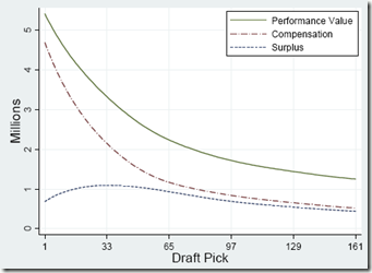
One of the unheralded elements to the Patriots’ success—perhaps rivaling Tom Brady himself in actual importance—is their penchant for stock-piling draft-picks in the “sweet spot” of the NFL draft (late 1st to mid-2nd round), where picks have the most surplus value. Once again, here’s the killer graph from the famous Massey-Thaler study on the topic:

In the 11 drafts since Belichick took over, the Patriots have made 17 picks between numbers 20 and 50 overall, the most in the NFL (the next-most is SF with 15, league average is obv 11). To illustrate how unusual their draft strategy has been, here’s a plot of their 2nd round draft position vs. their total wins over the same period:

Despite New England having the highest win percentage (not to mention most Super Bowl wins and appearances) over the period, there are 15 teams with lower average draft positions in the 2nd round. For comparison, they have the 2nd lowest average draft position in the 1st round and 7th lowest in the third.

Of course, the new collective bargaining agreement includes a rookie salary scale. Without going into all the details (in part because they’re extremely complicated and not entirely public), the key points are that it keeps total rookie compensation relatively stable while flattening the scale at the top, reducing guaranteed money, and shortening the maximum number of years for each deal.

These changes should all theoretically flatten out the “value curve” above. Here’s a rough sketch of what the changes seem to be attempting:

Since the original study was published, the dollar values have gone up and the top end has gotten more skewed. I adjusted the Y-axis to reflect the new top, but didn’t adjust the curve itself, so it should actually be somewhat steeper than it appears.  I tried to make the new curves as conceptually accurate as I could, but they’re not empirical and should be considered more of an “artist’s rendition” of what I think the NFL is aiming for.

With a couple of years of data, this should be a very interesting issue to revisit.  But, for now, I think it’s unlikely that the curve will actually be flattened very much. If I had to guess, I think it may end up “dual-peaked”: By far the greatest drop in guaranteed money will be for top QB prospects taken with the first few picks. These players already provide the most value, and are the main reason the original M/T performance graph inclines so steeply on the left. Additionally, they provide an opportunity for continued surplus value beyond the length of the initial contract. This should make the top of the draft extremely attractive, at least in years with top QB prospects.

On the other hand, I think the bulk of the effect on the rest of the surplus-value curve will be to shift it to the left. My reasons for thinking this are much more complicated, and include my belief that the original Massey/Thaler study has problems with its valuation model, but the extremely short version is that I have reason to believe that people systematically overvalue upper/middle 1st round picks.

How the Patriots Responded

Since I’ve been following the Patriots’ 2nd-round-oriented drafting strategy for years now, naturally my first thoughts after seeing the details of the new deal went to how this could kill their edge. Here’s a question I tweeted at the Sloan conference:

Actually, my concern about the Patriots drafting strategy was two-fold:

  1. The Patriots favorite place to draft could obviously lose its comparative value under the new system. If they left their strategy as-is, it could lead to their picking sub-optimally. At the very least, it should eliminate their exploitation opportunity.
  2. Though a secondary issue for this post, at some point  taking an extreme bang-for-your-buck approach to player value can run into diminishing returns and cause stagnation. Since you can only have so many players on your roster or on the field at a time, your ability to hoard and exploit “cheap” talent is constrained. This is a particularly big concern for teams that are already pretty good, especially if they already have good “value” players in a lot of positions: At some point, you need players who are less cheap but higher quality, even if their value per dollar is lower than the alternative.

Of course, if you followed the draft, you know that the Patriots, entering the draft with far fewer picks than usual, still traded up in the 1st round, twice.

Taken out of context, these moves seem extremely out of character for the Patriots. Yet the moves are perfectly consistent with an approach that understands and attacks my concerns: Making fewer, higher-quality picks is essentially the correct solution, and if the value-curve has indeed shifted up as I expect it has, the new epicenter of the Patriots’ draft activity may be directly on top of the new sweet spot.

Baseball

The entire affair reminds me of an old piece of poker wisdom that goes something like this: In a mixed game with one truly expert poker player and a bunch of completely outclassed amateurs, the expert’s biggest edge wouldn’t come in the poker variant with which he has the most expertise, but in some ridiculous spontaneous variant with tons of complicated made-up rules.

I forget where I first read the concept, but I know it has been addressed in various ways by many authors, ranging from Mike Caro to David Sklansky. I believe it was the latter (though please correct me if I’m wrong), who specifically suggested a Stud variant some of us remember fondly from childhood:

Several different games played only in low-stakes home games are called Baseball, and generally involve many wild cards (often 3s and 9s), paying the pot for wild cards, being dealt an extra upcard upon receiving a 4, and many other ad-hoc rules (for example, the appearance of the queen of spades is called a “rainout” and ends the hand, or that either red 7 dealt face-up is a rainout, but if one player has both red 7s in the hole, that outranks everything, even a 5 of a kind). These same rules can be applied to no peek, in which case the game is called “night baseball”.

The main ideas are that A) the expert would be able to adapt to the new rules much more quickly, and B) all those complicated rules make it much more likely that he would be able to find profitable exploitations (for Baseball in particular, there’s the added virtue of having several betting rounds per hand).

It will take a while to see how this plays out, and of course the abnormal outcome could just be a circumstances-driven coincidence rather than an explicit shift in the Patriots’ approach. But if my intuitions about the situation are right, Belichick may deserve extra credit for making deft adjustments in a changing landscape, much as you would expect from the Baseball-playing shark.

Graph of the Day: Quarterbacks v. Coaches, Draft Edition

[Note: With the recent amazing addition to my office, I’ve considered just turning this site into a full-on baby photo-blog (much like my Twitter feed).  While that would probably mean a more steady stream of content, it would also probably require a new name, a re-design, and massive structural changes.  Which, in turn, would raise a whole bevy of ontological issues that I’m too tired to deal with at the moment. So I guess back to sports analysis!]

In “A History of Hall of Fame QB-Coach Entanglement,” I talked a bit about the difficulty of “detangling” QB and coach accomplishments.  For a slightly more amusing historical take, here’s a graph illustrating how first round draft picks have gotten a much better return on investment (a full order of magnitude better vs. non-#1 overalls) when traded for head coaches than when used to draft quarterbacks:

Note: Since 1950. List of #1 Overall QB’s is here.  Other 1st Round QB’s here.  Other drafted QB’s here.  Super Bowl starters here.  QB’s that were immediately traded count for the team that got them.

Note*: . . that I know of. I googled around looking for coaches that cost their teams at least one first round draft pick to acquire, and I could only find 3: Bill Parcells (Patriots -> Jets), Bill Belichick (Jets -> Patriots), and Jon Gruden (Raiders -> Bucs).  If I’m missing anyone, please let me know.

Sample, schmample.

But seriously, the other 3 bars are interesting too.

Graph of the Day: Alanis Loves Rookie Quarterbacks

Last season I did some analysis of rookie starting quarterbacks and which of their stats are most predictive of future NFL success. One of the most fun and interesting results I found is that rookie interception % is a statistically significant positive indicator—that is, all else being equal, QB’s who throw more interceptions as rookies tend to have more successful careers.  I’ve been going back over this work recently with an eye towards posting something on the blog (coming soon!), and while playing around with examples I stumbled into this:

Note: Data points are QB’s in the Super Bowl era who were drafted #1 overall and started at least half of their team’s games as rookies (excluding Matthew Stafford and Sam Bradford for lack of ripeness). Peyton Manning and Jim Plunkett each threw 4.9% interceptions and won one Super Bowl, so I slightly adjusted their numbers to make them both visible, though the R-squared value of .7287 is accurate to the original (a linear trend actually performs slightly better—with an R-squared of .7411—but I prefer the logarithmic one aesthetically).

Notice the relationship is almost perfectly ironic: Excluding Steve Bartowski (5.9%), no QB with a lower interception percentage has won more Super Bowls than any QB with a higher one. Overall (including Steve B.), the seven QB’s with the highest rates have 12 Super Bowl rings, or an average of 1.7 per (and obv the remaining six have none).  And it’s not just Super Bowls: those seven also have 36 career Pro Bowl selections between them (average of 5.1), to just seven for the remainder (average of 1.2).

As for significance, obviously the sample is tiny, but it’s large enough that it would be an astounding statistical artifact if there were actually nothing behind it (though I should note that the symmetricality of the result would be remarkable even with an adequate explanation for its “ironic” nature).  I have some broader ideas about the underlying dynamics and implications at play, but I’ll wait to examine those in a more robust context. Besides, rank speculation is fun, so here are a few possible factors that spring to mind:

  1. Potential for selection effect: Most rookie QB’s who throw a lot of interceptions get benched.  Teams may be more likely to let their QB continue playing when they have more confidence in his abilities—and presumably such confidence correlates (at least to some degree) with actually having greater abilities.
  2. The San Antonio gambit: Famously, David Robinson missed most of the ’96-97 NBA season with back and foot injuries, allowing the Spurs to bomb their way into getting Tim Duncan, sending the most coveted draft pick in many years to a team that, when healthy, was already somewhat of a contender (also preventing a drool-worthy Iverson/Duncan duo in Philadelphia).  Similarly, if a quality QB prospect bombs out in his rookie campaign—for whatever reason, including just “running bad”—his team may get all of the structural and competitive advantages of a true bottom-feeder (such as higher draft position), despite actually having 1/3 of a quality team (i.e., a good quarterback) in place.
  3. Gunslingers are just better:  This is my favorite possible explanation, natch.  There are a lot of variations, but the most basic idea goes like this: While ultimately a good QB on a good team will end up having lower interception rates, interceptions are not necessarily bad.  Much like going for it on 4th down, often the best win-maximizing choice that a QB can make is to “gamble”—that is, to risking turning the ball over when the reward is appropriate. This can be play-dependent (like deep passes with high upsides and low downsides), or situation-dependent (like when you’re way behind and need to give yourself the chance to get lucky to have a chance to win).  E.g.: In defense of Brett Favre—who, in crunch time, could basically be counted on to deliver you either a win or multiple “ugly” INT’s—I’ve quipped: If a QB loses a game without throwing 4 interceptions, he probably isn’t trying hard enough.  And, of course, this latter scenario should come up a lot for the crappy teams that just drafted #1 overall:  I.e., when your rookie QB is going 4-12 and isn’t throwing 20 interceptions, he’s probably doing something wrong.

[Edit (9/24/2011) to add: Considering David Meyer’s comment below, I thought I should make clear that, while my interests and tastes lie with #3 above, I don’t mean to suggest that I endorse it as the most likely or most significant factor contributing to this particular phenomenon (or even the broader one regarding predictivity of rookie INT%).  While I do find it meaningful and relevant that this result is consistent with and supportive of some of my wilder thoughts about interceptions, risk-taking, and quarterbacking, overall I think that macroscopic factors are more likely to be the driving force in this instance.]

For the record, here are the 13 QB’s and their relevant stats:

[table “7” not found /]

Quick Take: Why Winning the NBA Draft Lottery Matters

Andres Alvarez (@NerdNumbers) tweeted the other day: “Opinion question. Does getting the #1 Pick in the Draft Lottery really up your odds at a title?”  To which I responded, “Yes, and it’s not close.”

If you’ve read my “How to Win a Championship in Any Sport,” you can probably guess why I would say that.  The reasoning is pretty simple:

  1. In any salary-capped sport, the key to building a championship contender is to maximize surplus value by underpaying your team as much as possible.
  2. The NBA is dominated by a handful of super-star players who get paid the same amount as regular-star players.
  3. Thus, the easiest way to get massive surplus value in the NBA is to get one or more of those players on your team, by any means necessary.
  4. Not only is the draft a great place to find potentially great players, but because of the ridiculously low rookie pay scale, your benefit to finding one is even greater.
  5. Superstars don’t grown on trees, and drafting #1 ensures you will get the player that you believe is most likely to become one.

I could leave it at that, as it’s almost necessarily true that drafting #1 will improve your chances.  But I suppose what people really want to know is how much does it “up your odds”?  To answer that, we also need to look at the empirical question of how valuable the “most likely to be a superstar” actually is.

Yes, #1 picks often bust out.  Yes, many great players are found in the other 59+ picks.  But it utterly confounds me why so many people seem to think that proving variance in outcomes means we shouldn’t pay attention to distribution of outcomes. [Side-note: It also bugs me that people think that because teams “get it wrong” so often, it must mean that NBA front offices are terrible at evaluating talent. This is logically false: maybe basketball talent is just extremely hard to evaluate!  If so, an incredible scouting department might be one that estimates an individual player’s value with slightly smaller error margins than everyone else—just as a roulette player who could guess the next number just 5% of the time could easily get rich. But I digress.]

So, on average, how much better are #1 draft picks than other high draft picks?  Let’s take a look at some data going back to 1969:

image

Ok, so #1 picks are, on average, a lot better than #2 picks, and it flattens out a bit from there.  For these purposes, I don’t think it’s necessary, but you can mess around with all the advanced stats and you’ll find pretty much the same thing (see, e.g., this old Arturo post). [Also, I won’t get into it here, but the flattening is important in its own right, as it tends to imply a non-linear talent distribution, which is consistent with my hypothesis that, unlike many other sports, basketball is dominated by extreme forces rather than small accumulated edges.]

So, a few extra points (or WPA’s, or WoW’s, or whatevers) here or there, what about championships?  And, specifically, what about championships a player wins for his drafting team?

image

Actually, this even surprised me: Knowing that Michael Jordan won 6 championships for his drafting team, I thought for sure the spike on pick 3 would be an issue.  But it turns out that the top picks still come out easily on top (and, again, the distribution among the rest is comparatively flat).  Also, it may not be obvious from that graph, but a higher proportion of their championships have gone to the teams that draft them as well.  So to recap (and add a little):

image

The bottom line is, at least over the last 40ish years, having the #1 pick in the draft was worth approximately four times as many championships as having a 2 through 8.  I would say that qualifies as “upping your odds.”

C.R.E.A.M. (Or, “How to Win a Championship in Any Sport”)

Does cash rule everything in professional sports?  Obviously it keeps the lights on, and it keeps the best athletes in fine bling, but what effect does the root of all evil have on the competitive bottom line—i.e., winning championships?

For this article, let’s consider “economically predictable” a synonym for “Cash Rules”:  I will use extremely basic economic reasoning and just two variables—presence of a salary cap and presence of a salary max in a sport’s labor agreement—to establish, ex ante, which fiscal strategies we should expect to be the most successful.  For each of the 3 major sports, I will then suggest (somewhat) testable hypotheses, and attempt to examine them.  If the hypotheses are confirmed, then Method Man is probably right—dollar dollar bill, etc.

Conveniently, on a basic yes/no grid of these two variables, our 3 major sports in the U.S. fall into 3 different categories:

image

So before treating those as anything but arbitrary arrangements of 3 letters, we should consider the dynamics each of these rules creates independently.  If your sport has a team salary cap, getting “bang for your buck” and ferreting out bargains is probably more important to winning than overall spending power.  And if your sport has a low maximum individual salary, your ability to obtain the best possible players—in a market where everyone knows their value but must offer the same amount—will also be crucial.  Considering permutations of thriftiness and non-economic acquisition ability, we end up with a simple ex ante strategy matrix that looks like this:

image

These one-word commandments may seem overly simple—and I will try to resolve any ambiguity looking at the individual sports below—but they are only meant to describe the most basic and obvious economic incentives that salary caps and salary maximums should be expected to create in competitive environments.

Major League Baseball: Spend

Hypothesis:  With free-agency, salary arbitration, and virtually no payroll restrictions, there is no strategic downside to spending extra money.  Combined with huge economic disparities between organizations, this means that teams that spend the most will win the most.

Analysis:  Let’s start with the New York Yankees (shocker!), who have been dominating baseball since 1920, when they got Babe Ruth from the Red Sox for straight cash, homey.  Note that I take no position on whether the Yankees filthy lucre is destroying the sport of Baseball, etc.  Also, I know very little about the Yankees payroll history, prior to 1988 (the earliest the USA Today database goes).  But I did come across this article from several years ago, which looks back as far as 1977.  For a few reasons, I think the author understates the case.  First, the Yankees low-salary period came at the tail end of a 12 year playoff drought (I don’t have the older data to manipulate, but I took the liberty to doodle on his original graph):

image

Note: Smiley-faces are Championship seasons.  The question mark is for the 1994 season, which had no playoffs.

Also, as a quirk that I’ve discussed previously, I think including the Yankees in the sample from which the standard deviation is drawn can be misleading: they have frequently been such a massive outlier that they’ve set their own curve.  Comparing the Yankees to the rest of the league, from last season back to 1988, looks like this:

image

Note: Green are Championship seasons.  Red are missed playoffs.

In 2005 the rest-of-league average payroll was ~$68 million, and the Yankees’ was ~$208 million (the rest-of-league standard deviation was $23m, but including the Yankees, it would jump to $34m).

While they failed to win the World Series in some of their most expensive seasons, don’t let that distract you:  money can’t guarantee a championship, but it definitely improves your chances.  The Yankees have won roughly a quarter of the championships over the last 20 years (which is, astonishingly, below their average since the Ruth deal).  But it’s not just them.  Many teams have dramatically increased their payrolls in order to compete for a World Series title—and succeeded! Over the past 22 years, the top 3 payrolls (per season) have won a majority of titles:

image

As they make up only 10% of the league, this means that the most spendy teams improved their title chances, on average, by almost a factor of 6.

National Basketball Association: Recruit (Or: “Press Your Bet”)

Hypothesis:  A fairly strict salary cap reigns in spending, but equally strict salary regulations mean many teams will enjoy massive surplus value by paying super-elite players “only” the max.  Teams that acquire multiple such players will enjoy a major championship advantage.

Analysis: First, in case you were thinking that the 57% in the graph above might be caused by something other than fiscal policy, let’s quickly observe how the salary cap kills the “spend” strategy: image

Payroll information from USA Today’s NBA and NFL Salary Databases (incidentally, this symmetry is being threatened, as the Lakers, Magic, and Mavericks have the top payrolls this season).

I will grant there is a certain apples-to-oranges comparison going on here: the NFL and NBA salary-cap rules are complex and allow for many distortions.  In the NFL teams can “clump” their payroll by using pro-rated signing bonuses (essentially sacrificing future opportunities to exceed the cap in the present), and in the NBA giant contracts are frequently moved to bad teams that want to rebuild, etc.  But still: 5%.  Below expectation if championships were handed out randomly.
And basketball championships are NOT handed out randomly.  My hypothesis predicts that championship success will be determined by who gets the most windfall value from their star player(s).  Fifteen of the last 20 NBA championships have been won by Kobe Bryant, Tim Duncan, or Michael Jordan.  Clearly star-power matters in the NBA, but what role does salary play in this?

Prior to 1999, the NBA had no salary maximum, though salaries were regulated and limited in a variety of ways.  Teams had extreme advantages signing their own players (such as Bird rights), but lack of competition in the salary market mostly kept payrolls manageable.  Michael Jordan famously signed a lengthy $25 million contract extension basically just before star player salaries exploded, leaving the Bulls with the best player in the game for a song (note: Hakeem Olajuwon’s $55 million payday came after he won 2 championships as well).  By the time the Bulls were forced to pay Jordan his true value, they had already won 4 championships and built a team around him that included 2 other All-NBA caliber players (including one who also provided extreme surplus value).  Perhaps not coincidentally, year 6 in the graph below is their record-setting 72-10 season:
image

Note: Michael Jordan’s salary info found here.  Historical NBA salary cap found here.

The star player salary situation caught the NBA off-guard.  Here’s a story from Time magazine in 1996 that quotes league officials and executives:

“It’s a dramatic, strategic judgment by a few teams,” says N.B.A. deputy commissioner Russ Granik. .
Says one N.B.A. executive: “They’re going to end up with two players making about two-thirds of the salary cap, and another pair will make about 20%. So that means the rest of the players will be minimum-salary players that you just sign because no one else wants them.” . . .
Granik frets that the new salary structure will erode morale. “If it becomes something that was done across the league, I don’t think it would be good for the sport,” he says.

What these NBA insiders are explaining is basic economics:  Surprise!  Paying better players big money means less money for the other guys.  Among other factors, this led to 2 lockouts and the prototype that would eventually lead to the current CBA (for more information than you could ever want about the NBA salary cap, here is an amazing FAQ).

The fact that the best players in the NBA are now being underpaid relative to their value is certain.  As a back of the envelope calculation:  There are 5 players each year that are All-NBA 1st team, while 30+ players each season are paid roughly the maximum.  So how valuable are All-NBA 1st team players compared to the rest?  Let’s start with: How likely is an NBA team to win a championship without one?

image

In the past 20 seasons, only the 2003-2004 Detroit Pistons won the prize without a player who was a 1st-Team All-NBAer in their championship year.
To some extent, these findings are hard to apply strategically.  All but those same Pistons had at least one home-grown All-NBA (1st-3rd team) talent—to win, you basically need the good fortune to catch a superstar in the draft.  If there is an actionable take-home, however, it is that most (12/20) championship teams have also included a second All-NBA talent acquired through trade or free agency: the Rockets won after adding Clyde Drexler, the second Bulls 3-peat added Dennis Rodman (All-NBA 3rd team with both the Pistons and the Spurs), the Lakers and Heat won after adding Shaq, the Celtics won with Kevin Garnett, and the Lakers won again after adding Pau Gasol.

Each of these players was/is worth more than their market value, in most cases as a result of the league’s maximum salary constraints.  Also, in most of these cases, the value of the addition was well-known to the league, but the inability of teams to outbid each other meant that basketball money was not the determinant factor in the players choosing their respective teams.  My “Recruit” strategy anticipated this – though it perhaps understates the relative importance of your best player being the very best.  This is more a failure of the “recruit” label than of the ex ante economic intuition, the whole point of which was that cap+max –> massive importance of star players.

National Football League: Economize (Or: “WWBBD?”)

Hypothesis:  The NFL’s strict salary cap and lack of contract restrictions should nullify both spending and recruiting strategies.  With elite players paid closer to what they are worth, surplus value is harder to identify.  We should expect the most successful franchises to demonstrate both cunning and wise fiscal policy.

Analysis: Having a cap and no max salaries is the most economically efficient fiscal design of any of the 3 major sports.  Thus, we should expect that massively dominating strategies to be much harder to identify.  Indeed, the dominant strategies in the other sports are seemingly ineffective in the NFL: as demonstrated above, there seems to be little or no advantage to spending the most, and the abundant variance in year-to-year team success in the NFL would seem to rule out the kind of individual dominance seen in basketball.

Thus, to investigate whether cunning and fiscal sense are predominant factors, we should imagine what kinds of decisions a coach or GM would make if his primary qualities were cunning and fiscal sensibility.  In that spirit, I’ve come up with a short list of 5 strategies that I think are more or less sound, and that are based largely on classically “economic” considerations:

1.  Beg, borrow, or steal yourself a great quarterback:
Superstar quarterbacks are probably underpaid—even with their monster contracts—thus making them a good potential source for surplus value.  Compare this:

Note: WPA (wins added) stats from here.

With this:

The obvious caveat here is that the entanglement question is still empirically open:  How much do good QB’s make their teams win v. How much do winning teams make their QB’s look good?  But really quarterbacks only need to be responsible for a fraction of the wins reflected in their stats to be worth more than what they are being paid. (An interesting converse, however, is this: the fact that great QB’s don’t win championships with the same regularity as, say, great NBA players, suggests that a fairly large portion of the “value” reflected by their statistics is not their responsibility).

2. Plug your holes with the veteran free agents that nobody wants, not the ones that everybody wants:
If a popular free agent intends to go to the team that offers him the best salary, his market will act substantially like a “common value” auction.  Thus, beware the Winner’s Curse. In simple terms: If 1) a player’s value is unknown, 2) each team offers what they think the player is worth, and 3) each team is equally likely to be right; then: 1) The player’s expected value will correlate with the average bid, and 2) the “winning” bid probably overpaid.

Moreover, even if the winner’s bid is exactly right, that just means they will have successfully gained nothing from the transaction.  Assuming equivalent payrolls, the team with the most value (greatest chance of winning the championship) won’t be the one that pays the most correct amount for its players, it will—necessarily—be the one that pays the least per unit of value.  To accomplish this goal, you should avoid common value auctions as much as possible!  In free agency, look for the players with very small and inefficient markets (for which #3 above is least likely to be true), and then pay them as little as you can get away with.

3. Treat your beloved veterans with cold indifference.
If a player is beloved, they will expect to be paid.  If they are not especially valuable, they will expect to be paid anyway, and if they are valuable, they are unlikely to settle for less than they are worth.  If winning is more important to you than short-term fan approval, you should be both willing and prepared to let your most beloved players go the moment they are no longer a good bargain.

4. Stock up on mid-round draft picks.
Given the high cost of signing 1st round draft picks, 2nd round draft picks may actually be more valuable.  Here is the crucial graph from the Massey-Thaler study of draft pick value (via Advanced NFL Stats):

image
The implications of this outcome are severe.  All else being equal, if someone offers you an early 2nd round draft pick for your early 1st round draft pick, they should be demanding compensation from you (of course, marginally valuable players have diminishing marginal value, because you can only have/play so many of them at a time).

5. When the price is right: Gamble.

This rule applies to fiscal decisions, just as it does to in-game ones.  NFL teams are notoriously risk-averse in a number of areas: they are afraid that someone after one down season is washed up, or that an outspoken player will ‘disrupt’ the locker room, or that a draft pick might have ‘character issues’.  These sorts of questions regularly lead to lengthy draft slides and dried-up free agent markets.  And teams are right to be concerned: these are valid possibilities that increase uncertainty.  Of course, there are other possibilities. Your free agent target simply may not be as good as you hope they are, or your draft pick may simply bust out.  Compare to late-game 4th-down decisions: Sometimes going for it on 4th down will cause you to lose immediately and face a maelstrom of criticism from fans and press, where punting or kicking may quietly lead to losing more often.  Similarly, when a team takes a high-profile personnel gamble and it fails, they may face a maelstrom of criticism from fans and press, where the less controversial choice might quietly lead to more failure.

The economizing strategy here is to favor risks when they are low cost but have high upsides.  In other words, don’t risk a huge chunk of your cap space on an uncertain free agent prospect, risk a tiny chunk of your cap space on an even more uncertain prospect that could work out like gangbusters.

Evaluation:

Now, if only there were a team and coach dedicated to these principles—or at least, for contrapositive’s sake, a team that seemed to embrace the opposite.

Oh wait, we have both!  In the last decade, Bill Belichick and the New England Patriots have practically embodied these principles, and in the process they’ve won 3 championships, have another 16-0/18-1 season, have set the overall NFL win-streak records, and are presently the #1 overall seed in this year’s playoffs. OTOH, the Redskins have practically embodied the opposite, and they have… um… not.
Note that the Patriots’ success has come despite a league fiscal system that allows teams to “load up” on individual seasons, distributing the cost onto future years (which, again, helps explain the extreme regression effect present in the NFL).  Considering the long odds of winning a Super Bowl—even with a solid contender—this seems like an unwise long-run strategy, and the most successful team of this era has cleverly taken the long view throughout.

Conclusions

The evidence in MLB and in the NBA is ironclad: Basic economic reasoning is extremely probative when predicting the underlying dynamics behind winning titles.  Over the last 20 years of pro baseball, the top 3 spenders in the league each year win 57% of the championships.  Over a similar period in basketball, the 5 (or fewer) teams with 1st-Team All-NBA players have won 95%.

In the NFL, the evidence is more nuance and anecdote than absolute proof.  However, our ex ante musing does successfully predict that neither excessive spending nor recruiting star players at any cost (excepting possibly quarterbacks) is a dominant strategy.

On balance, I would say that the C.R.E.A.M. hypothesis is substantially more supported by the data than I would have guessed.

The 1-15 Rams and the Salary Cap—Watch Me Crush My Own Hypothesis

It is a quirky little fact that 1-15 teams have tended to bounce back fairly well.  Since expanding to 16 games in 1978, 9 teams have hit the ignoble mark, including last year’s St. Louis Rams.  Of the 8 that did it prior to 2009, all but the 1980 Saints made it back to the playoffs within 5 years, and 4 of the 8 eventually went on to win Super Bowls, combining for 8 total.  The median number of wins for a 1-15 team in their next season is 7:

1-15 teams_23234_image001

1-15 teams_23234_image003

My grand hypothesis about this was that the implementation of the salary cap after the 1993-94 season, combined with some of the advantages I discuss below (especially 2 and 3), has been a driving force behind this small-but-sexy phenomenon: note that at least for these 8 data points, there seems to be an upward trend for wins and downward trend for years until next playoff appearance.  Obviously, this sample is way too tiny to generate any conclusions, but before looking at harder data, I’d like to speculate a bit about various factors that could be at play.  In addition to normally-expected regression to the mean, the chain of consequences resulting from being horrendously bad is somewhat favorable:

  1. The primary advantages are explicitly structural:  Your team picks at the top of each round in the NFL draft.  According to ESPN’s “standard” draft-pick value chart, the #1 spot in the draft is worth over twice as much as the 16th pick [side note: I don’t actually buy this chart for a second.  It massively overvalue 1st round picks and undervalues 2nd round picks, particularly when it comes to value added (see a good discussion here)]:image
  2. The other primary benefit, at least for one year, comes from the way the NFL sets team schedules: 14 games are played in-division and against common divisional opponents, but the last two games are set between teams that finished in equal positions the previous year (this has obviously changed many times, but there have always been similar advantages).  Thus, a bottom-feeder should get a slightly easier schedule, as evidenced by the Rams having the 2nd-easiest schedule for this coming season.
  3. There are also reliable secondary benefits to being terrible, some of which get greater the worse you are.  A huge one is that, because NFL statistics are incredibly entangled (i.e., practically every player on the team has an effect on every other player’s statistics), having a bad team tends to drag everyone’s numbers down.  Since the sports market – and the NFL’s in particular – is stats-based on practically every level, this means you can pay your players less than what they’re worth going forward.  Under the salary cap, this leaves you more room to sign and retain key players, or go for quick fixes in free agency (which is generally unwise, but may boost your performance for a season or two).
  4. A major tertiary effect – one that especially applies to 1-15 teams, is that embarrassed clubs tend to “clean house,” meaning, they fire coaches, get rid of old and over-priced veterans, make tough decisions about star players that they might not normally be able to make, etc.  Typically they “go young,” which is advantageous not just for long-term team-building purposes, but because young players are typically the best value in the short term as well.
  5. An undervalued quaternary effect is that new personnel and new coaching staff, in addition to hopefully being better at their jobs than their predecessors, also make your team harder to prepare for, just by virtue of being new (much like the “backup quarterback effect,” but for your whole team).
  6. A super-important quinary effect is that. . .  Ok, sorry, I can’t do it.

Of course, most of these effects are relevant to more than just 1-15 teams, so perhaps it would be better to expand the inquiry a tiny bit.  For this purpose, I’ve compiled the records of every team since the merger, so beginning in 1970, and compared them to their record the following season (though it only affects one data point, I’ve treated the first Ravens season as a Browns season, and treated the new Browns as an expansion team).  I counted ties as .5 wins, and normalized each season to 16 games (and rounded).  I then grouped the data by wins in the initial season and plotted it on a “3D Bubble Chart.”  This is basically a scatter-plot where the size of each data-point is determined by the number of examples (e.g., only 2 teams have gone undefeated, so the top-right bubble is very small).  The 3D is not just for looks: the size of each sphere is determined by using the weights for volume, which makes it much less “blobby” than 2D, and it allows you to see the overlapping data points instead of just one big ink-blot:

season wins_31685_image001

*Note: again, the x-axis on this graph is wins in year n, and the y axis is wins in year n+1. Also, note that while there are only 16 “bubbles,” they represent well over a thousand data points, so this is a fairly healthy sample.

The first thing I can see is that there’s a reasonably big and fat outlier there for 1-15 teams (the 2nd bubble from the left)!  But that’s hardly a surprise considering we started this inquiry knowing that group had been doing well, and there are other issues at play: First, we can see that the graph is strikingly linear.  The equation at the bottom means that to predict a team’s wins for one year, you should multiply their previous season’s win total by ~.43 and add ~4.7 (e.g.’s: an 8-win team should average about 8 wins the next year, a 4-win team should average around 6.5, and a 12-win team should average around 10).  The number highlighted in blue tells you how important the previous season’s win’s are as a predictor: the higher the number, the more predictive.

So naturally the next thing to see is a breakdown of these numbers between the pre- and post-salary cap eras:

season wins_31685_image003

season wins_31685_image005

Again, these are not small sample-sets, and they both visually and numerically confirm that the salary-cap era has greatly increased parity: while there are still plenty of excellent and terrible teams overall, the better teams regress and the worse teams get better, faster.  The equations after the split lead to the following predictions for 4, 8, and 12 win teams (rounded to the nearest .25):

W Pre-SC Post-SC
4 6.25 7
8 8.25 8
12 10.5 9.25
Yes, the difference in expected wins between a 4-win team and a 12-win team in the post-cap era is only just over 2 wins, down from over 4.

While this finding may be mildly interesting in its own right, sadly this entire endeavor was a complete and utter failure, as the graphs failed to support my hypothesis that the salary cap has made the difference for 1-15 teams specifically.  As this is an uncapped season, however, I guess what’s bad news for me is good news for the Rams.